REVIEW 2 major objections 5 minor 27 references
Conditioning multivariate extremes on arbitrary half-spaces yields directional variograms whose ensembles cut estimation variance while trading bias against half-space mass.
Reviewed by Pith at T0; open to challenge. T0 means a machine referee read the full paper against a public rubric. the ladder, T0–T4 →
T0 review · grok-4.5
2026-07-12 03:28 UTC pith:RTW2XFDA
load-bearing objection Clean, usable generalization of extremal variograms to arbitrary half-spaces, with solid theory and a clear bias–variance picture for HR. the 2 major comments →
Directional variograms for multivariate extremes
The pith
A machine-rendered reading of the paper's core claim, the machinery that carries it, and where it could break.
Core claim
For any direction v in the probability simplex the conditioned multivariate generalized Pareto vector admits the decomposition Y^v =^d W^v + E 1, where W^v is the v-extremal function on v^perp and E is independent standard exponential; the associated v-variogram equals the Hüsler–Reiss parameter matrix for every v, admits closed forms for logistic and Dirichlet models, and its empirical ensembles improve mean-squared error by exploiting the bias–variance trade-off controlled by half-space mass.
What carries the argument
The v-extremal function W^v obtained by oblique projection of the half-space-conditioned vector Y^v (or equivalently by exponential tilting of a generator), which carries the entire dependence structure of the v-variogram and links densities across directions by exponential tilting.
Load-bearing premise
Thresholded, empirically margin-transformed samples behave like exact draws from the limiting multivariate generalized Pareto law, and the reported bias–variance patterns transfer beyond Hüsler–Reiss dependence.
What would settle it
In a high-dimensional simulation from a non-Hüsler–Reiss domain-of-attraction model, check whether ensembles of empirical v-variograms still reduce MSE relative to the classical single-component average once the threshold is varied; systematic failure would refute the claimed generality of the bias–variance mechanism.
If this is right
- Practitioners can replace the classical average of d axis-aligned extremal variograms by a weighted or unweighted ensemble over any collection of directions, with expected variance reduction from overlapping half-spaces.
- The resistance-curvature direction v0 (or its simplex projection) supplies a canonical low-bias estimator whose half-space contains the fewest expected exceedances.
- New closed-form Hüsler–Reiss densities parameterized by arbitrary v simplify likelihood construction and graphical-model inference.
- Bias-dominated low-threshold regimes favor directions of small half-space mass; variance-dominated high-threshold regimes favor unit vectors.
- Logistic and Dirichlet models obtain explicit v-dependent variogram formulae usable for moment matching or goodness-of-fit.
Where Pith is reading between the lines
- The same half-space geometry should extend immediately to other summary statistics (extremal coefficients, madograms, tail dependence functions) that are currently computed only on axis-aligned exceedances.
- Because half-space mass is a continuous function of v, one can treat direction choice itself as a continuous tuning parameter and optimize it by cross-validation on held-out extremes.
- The resistance-curvature vector links the statistical construction to discrete curvature of Euclidean distance matrices, suggesting that geometric invariants of the variogram may systematically control estimation efficiency.
Editorial analysis
A structured set of objections, weighed in public.
Referee Report
Summary. The paper generalizes the extremal variogram of Engelke and Volgushev (2022) by conditioning a multivariate generalized Pareto vector Y on arbitrary half-spaces H_v = {y : v^T Y > 0} for v in the probability simplex. It defines Y^v = (Y | v^T Y > 0) and the v-variogram Gamma^v_ij = Var(Y_i^v - Y_j^v), proves the decomposition Y^v =^d W^v + E 1 with W^v the v-extremal function on v^perp and E independent Exp(1), and relates the laws of Y^v and W^v across directions via exponential tilting. Closed forms for Gamma^v are obtained for logistic, Dirichlet, and Husler-Reiss models; for HR, Gamma^v equals the parameter matrix for every v, new density representations are derived, and the resistance-curvature vector v0 is shown to center W^{v0} and minimize half-space mass Lambda(H_v). Empirical v-variograms and ensemble averages over collections V are introduced, and simulations (mainly HR limits and domain-of-attraction data) document a bias-variance trade-off driven by Lambda(H_v) and variance reduction from ensembles.
Significance. The work cleanly extends a standard dependence summary for multivariate extremes from axis-aligned conditioning to general half-spaces, with complete proofs of the stochastic representations, tilting identities, and closed forms (Appendix C). The HR density formulae and the characterization of v0 (least-mass half-space and centered Gaussian extremal function) are new and link extremal statistics to Euclidean-distance / resistance geometry. The simulation study is carefully designed (M=2000, fixed and random Gamma, multiple thresholds and ensemble constructions) and shows that ensembles can improve MSE relative to the classical average of unit-vector variograms. Strengths include full proofs, recovery of known special cases, and transparent scoping of the statistical claims to HR-type settings. The contribution is solid and useful for inference and graphical modeling of extremes.
major comments (2)
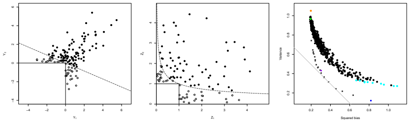
- Section 5 and Figures 6-10: the bias-variance and ensemble conclusions are demonstrated only for Husler-Reiss limits and max-stable HR data in the domain of attraction. Because Gamma^v is independent of v only for HR (Example 3.13), the practical recommendation to average over multiple v is less clear for logistic or Dirichlet models, where Gamma^v itself depends on v. A short simulation or discussion for at least one non-HR family would make the statistical claims more transferable; without it the ensemble gains remain HR-specific.
- Definition 3.9 and Section 5.1: existence of Gamma^v requires finite second moments of component differences under every half-space conditioning. This is the same regularity used for classical extremal variograms and holds for the three parametric families treated, but the paper does not state sufficient conditions on the exponent measure (or generator) that guarantee these moments for general Y. A brief remark on when the empirical v-variogram is well-defined would strengthen the general theory.
minor comments (5)
- Notation: the paper uses both Lambda_d and Delta^{d-1} for the simplex in places (e.g., Example 3.13 vs. Section 2.1); unify to one symbol.
- Figure 1 (right) and Table 1: the ensemble constructions are clear in the text but the figure legend could name the two ensembles more explicitly (e.g., {e1,e2} vs. 11-point grid).
- Remark 4.8 / Eq. (4.4): the convex program for v0* when v0 has negative entries is well-motivated; a one-line note that standard QP solvers suffice would help practitioners.
- Appendix B: the Hausdorff-measure convention for densities on hyperplanes is carefully defined; a forward reference from Lemma 3.6 / Proposition 3.8 would help readers who skip the appendix.
- Typos: 'H¨ usler' spacing and occasional missing spaces after commas in the arXiv text; also 'Lambda_d' vs. 'Delta' inconsistency noted above.
Circularity Check
No significant circularity: directional objects and closed forms are derived from standard MGP constructions with complete proofs; simulations compare estimators to known generated truth.
full rationale
The paper defines Y^v and Γ^v, then proves the decomposition Y^v =^d W^v + E1 (Prop. 3.2), generator/tilting relations (Prop. 3.3–3.8), and closed-form Γ^v for logistic, Dirichlet, and Hüsler–Reiss models (Ex. 3.11–3.13) from standard exponent-measure and generator constructions; full proofs appear in Appendix C. For HR, Γ^v = Γ for all v is a derived invariance of the Gaussian generator under tilting and projection, not an input. Density formulas and the resistance-curvature characterization of v0 (Prop. 4.3, Cor. 4.6–4.7) follow algebraically from those representations. Empirical ˆΓ^v and ensembles are sample analogues; the simulation study evaluates them against known generated Γ matrices under HR limits and domain-of-attraction data, not fitted targets relabeled as predictions. Self-citations (Engelke–Volgushev 2022, Engelke–Hitz 2020, Hentschel et al. 2025) supply background objects being generalized; they are not uniqueness theorems that force the new claims. No step reduces a claimed derivation to its own definition or fit by construction.
Axiom & Free-Parameter Ledger
free parameters (3)
- threshold quantile p
- direction set V for ensemble estimator
- sparsity / face sampling of candidate v
axioms (6)
- domain assumption X lies in the domain of attraction of a multivariate generalized Pareto Y with standard exponential margins (limit (2.1) exists).
- domain assumption Componentwise differences under half-space conditioning have finite variance so that Γ^v is well-defined.
- domain assumption For v in the probability simplex, H_v is contained in the MGP support L = {x : x ≰ 0}.
- domain assumption Hüsler–Reiss parameter Γ is conditionally negative definite with zero diagonal and positive off-diagonals (Γ ∈ D).
- standard math Densities of vectors supported on hyperplanes are taken w.r.t. (d−1)-dimensional Hausdorff measure (Definition B.1).
- domain assumption Empirical marginal transforms and fixed high exponential quantile qp produce samples approximately distributed as Y.
invented entities (3)
-
v-variogram Γ^v
independent evidence
-
v-extremal function W^v
independent evidence
-
Resistance-curvature direction v0 used as least-mass / centering half-space for HR
independent evidence
Cite this review
Pith. "Pith review of Directional variograms for multivariate extremes." pith.science (2026). https://pith.science/paper/RTW2XFDA
@misc{pith2026260703290,
  author       = {Pith},
  title        = {Pith review of: Directional variograms for multivariate extremes},
  year         = {2026},
  howpublished = {\url{https://pith.science/paper/RTW2XFDA}},
  note         = {Machine review of arXiv:2607.03290}
}
read the original abstract
Multivariate generalized Pareto distributions arise as limits of threshold exceedances and form a central model class for multivariate extremes. Existing inference methods based on the extremal variogram condition on the value of a single component, which can be statistically suboptimal. We generalize this approach by conditioning the multivariate generalized Pareto random vector $Y$ to lie on arbitrary half-spaces. Specifically, for a direction vector $v$, we introduce the random vector $Y^v = (Y \mid v^\top Y > 0)$ and define the associated $v$-variogram $\Gamma_{ij}^v=\mathrm{Var}(Y_i^v-Y_j^v)$. We establish the decomposition $Y^v \stackrel{d}{=} W^v+E\mathbf{1}$ into the so-called $v$-extremal function $W^v$ and an independent exponential random variable $E$, and derive several results relating these random variables to each other. For logistic, Dirichlet, and H\"usler-Reiss multivariate generalized Pareto models, we derive closed-form expressions for $\Gamma^v$. In the H\"usler-Reiss case, we further derive new density representations and identify a distinguished resistance-curvature vector $v_0$ that uniquely centers the Gaussian law of $W^{v_0}$ while characterizing the least-mass half-space. On the statistical side, we introduce empirical $v$-variograms and show in a simulation study that the choice of $v$ induces a pronounced bias-variance trade-off that is strongly related to the mass of the conditioning half-space. Moreover, combining information across multiple directions $v$ can substantially reduce estimation variance relative to methods based on a single vector.
Figures


Reference graph
Works this paper leans on
-
[1]
Bolin, D., Braunsteins, P., Engelke, S., and Huser, R. (2025). Intrinsic W hittle-- M at\'ern fields and sparse spatial extremes. https://arxiv.org/abs/2512.23395
arXiv 2025
-
[2]
Coles, S. G. and Tawn, J. A. (1991). Modelling extreme multivariate events. J. R. Stat. Soc. Ser. B. Stat. Methodol. , 53(2):377--392
1991
-
[3]
and Strokorb, K
Corradini, M. and Strokorb, K. (2024). Stochastic ordering in multivariate extremes. Extremes , 27(3):357--396
2024
-
[4]
Devriendt, K. (2022). Graph geometry from effective resistances . PhD thesis, University of Oxford
2022
-
[5]
Devriendt, K., Echave-Sustaeta Rodríguez , I., and Röttger, F. (2026). Extremal conditional independence for H \"usler- R eiss distributions via modular functions. https://arxiv.org/abs/2601.21931
arXiv 2026
-
[6]
Dombry, C., Engelke, S., and Oesting, M. (2016). Exact simulation of max-stable processes. Biometrika , 103:303--317
2016
-
[7]
Dombry, C., Eyi-Minko, F., and Ribatet, M. (2013). Conditional simulation of max-stable processes. Biometrika , 100(1):111--124
2013
-
[8]
and Huang, X
Drees, H. and Huang, X. (1998). Best attainable rates of convergence for estimators of the stable tail dependence function. Journal of Multivariate Analysis , 64(1):25--46
1998
-
[9]
Einmahl, J. H. J. and Segers, J. (2009). Maximum empirical likelihood estimation of the spectral measure of an extreme-value distribution. Ann. Statist. , 37(5B):2953--2989
2009
-
[10]
Engelke, S., Gnecco, N., and Röttger, F. (2025). Extremes of structural causal models. https://arxiv.org/abs/2503.06536
Pith/arXiv arXiv 2025
-
[11]
Engelke, S., Hentschel, M., Lalancette, M., and R\" o ttger, F. (2024a). Graphical models for multivariate extremes. https://arxiv.org/abs/2402.02187
-
[12]
and Hitz, A
Engelke, S. and Hitz, A. S. (2020). Graphical models for extremes (with discussion). J. R. Stat. Soc. Ser. B Stat. Methodol , 82(4):871--932
2020
-
[13]
S., Gnecco, N., and Hentschel, M
Engelke, S., Hitz, A. S., Gnecco, N., and Hentschel, M. (2024b). graphicalExtremes: Statistical Methodology for Graphical Extreme Value Models . R package version 0.3.3
-
[14]
Engelke, S., Malinowski, A., Kabluchko, Z., and Schlather, M. (2015). Estimation of H üsler- R eiss distributions and B rown- R esnick processes. J. R. Stat. Soc. Ser. B Stat. Methodol , 77(1):239--265
2015
-
[15]
and Volgushev, S
Engelke, S. and Volgushev, S. (2022). Structure learning for extremal tree models. Journal of the Royal Statistical Society Series B: Statistical Methodology , 84(5):2055--2087
2022
-
[16]
Gower, J. (1982). Euclidean distance geometry. Math. Scientist , 7:1--14
1982
-
[17]
Halliwell, L. J. (2021). The Log - Gamma Distribution and Non - Normal Error . Variance , 13(2):173--189
2021
-
[18]
Hentschel, M., Engelke, S., and Segers, J. (2025). Statistical inference for H üsler–- R eiss graphical models through matrix completions. Journal of the American Statistical Association , 120(550):909--921
2025
-
[19]
and Reiss, R.-D
H \"u sler, J. and Reiss, R.-D. (1989). Maxima of normal random vectors: Between independence and complete dependence . Statist. Prob. Letters , 7(4):283--286
1989
-
[20]
Kiriliouk, A., Rootz\'en, H., Segers, J., and Wadsworth, J. L. (2018). Peaks over thresholds modeling with multivariate generalized Pareto distributions. Technometrics , 61:123--135
2018
-
[21]
Resnick, S. I. (2008). Extreme Values, Regular Variation, and Point Processes , volume 4. Springer Science & Business Media
2008
-
[22]
Rootz\'en, H., Segers, J., and Wadsworth, J. L. (2018). Multivariate generalized Pareto distributions: Parametrizations, representations, and properties. J. Multivariate Anal. , 165:117--131
2018
-
[23]
and Tajvidi, N
Rootz \'e n, H. and Tajvidi, N. (2006). Multivariate generalized P areto distributions. Bernoulli , 12:917--930
2006
-
[24]
Röttger, F., Engelke, S., and Zwiernik, P. (2023). Total positivity in multivariate extremes . Ann. Statist. , 51(3):962 -- 1004
2023
-
[25]
Segers, J. (2020). One- versus multi-component regular variation and extremes of Markov trees. Adv. in Appl. Probab. , 52:855--878
2020
-
[26]
and Tawn, J
Wadsworth, J. and Tawn, J. (2014). Efficient inference for spatial extreme value processes associated to log- Gaussian random functions. Biometrika , 101(1):1--15
2014
-
[27]
Wan, P. (2026). Characterizing extremal dependence on a hyperplane. Biometrika , 113(2):asag015
2026
discussion (0)
Sign in with ORCID, Apple, or X to comment. Anyone can read and Pith papers without signing in.