REVIEW 5 major objections 4 minor 33 references
Quasar photometric redshifts cannot be trusted without multi-component uncertainty models.
Reviewed by Pith at T0; open to challenge. T0 means a machine referee read the full paper against a public rubric. the ladder, T0–T4 →
For KiDS quasars, multi-component MDNs and BNNs reconstruct redshift distributions better than plain ANNs, but the best model depends on the data-quality regime and combined faint/missing-band cases degrade all models.
T0 review reviewed 2026-08-04 challenge →
load-bearing objection The body is a useful, internally consistent benchmark of quasar photo-z uncertainty models, but the arXiv abstract contradicts its own Table 2 and promises an SOM/PIT analysis that the text doesn't deliver. the 5 major comments →
Quasar photometric redshifts beyond the spectroscopic coverage: Uncertainty models and redshift distributions in the Kilo-Degree Survey DR5
The pith
A machine-rendered reading of the paper's core claim, the machinery that carries it, and where it could break.
The reading
Core claim
The central claim is that an accurate reconstruction of the true redshift distribution is unattainable without a proper uncertainty estimation framework, and that MDNs with at least two Gaussian components are essential to capture the intrinsic multi-modality of photo-z solutions. Concretely, on a clean random test set the ANN's distribution reconstruction error is about six times that of the best MDN; the single-Gaussian MDN is miscalibrated and produces more catastrophic outliers than the ANN. A three-component MDN is the best MDN overall, while a three-component BNN improves the negative log-likelihood by 0.11 on faint extrapolation data but is 0.07 worse for brighter objects. In the hard
What carries the argument
The load-bearing object is the Gaussian Mixture Model output layer attached to a neural network (MDN) or to a Bayesian network (BNN), which turns photo-z prediction into a full probability density function rather than a point estimate. The paper compares these PDFs through the negative log-likelihood at the true spectroscopic redshift, and reconstructs the redshift distribution by Monte Carlo sampling each predicted PDF. The BNN estimates epistemic uncertainty by averaging 100 stochastic forward passes. A separate diagnostic uses t-SNE and HDBSCAN clustering on the sampled PDF values to expose degenerate solutions.
Load-bearing premise
The DESI DR1 spectroscopic quasars matched to KiDS are treated as an unbiased ground truth for the faint and missing-band test sets; if DESI target selection, redshift failures, or the 1-arcsec cross-match correlate with r>22.9 or missing u-band, the reported model rankings and n(z) reconstructions reflect selection effects rather than model capability.
What would settle it
Take a spectroscopically complete sample of faint quasars from a deeper survey that does not depend on DESI targeting, and repeat the faint-extrapolation NLL comparison between the three-component MDN and BNN. If the BNN's 0.11 NLL advantage disappears, the reported benefit of Bayesian networks is an artifact of the DESI selection function. A second test: recompute the 'missing features' rankings after dropping objects with missing u-band; if the rankings change, the results are driven by the imputation of the most important band.
If this is right
- Tomographic analyses with photometric quasars should be based on predicted probability distributions, not on single point estimates, since the ANN's reconstructed n(z) shows step-like artifacts and six times the error of the best uncertainty-aware model.
- At least two Gaussian mixture components are required in the output layer; a single Gaussian is miscalibrated and yields more catastrophic outliers than a plain ANN.
- Bayesian neural networks with three components are the best choice for samples extending fainter than the training set (NLL gain 0.11), but they come with a 0.07 NLL penalty for well-covered bright sources.
- Reconstruction remains feasible for fainter data or missing magnitudes separately, but fails when both occur together, so survey samples must be quality-controlled for combined incompleteness.
- Clustering predicted photo-z PDFs can identify degenerate redshift pairs ((1.2,2.3) and (1.6,2.5)) that could be removed from cosmological inference.
Where Pith is reading between the lines
- Because 76% of missing-band cases are missing the u-band, the paper's grouped 'missing features' test is effectively a u-band dropout test; a per-band analysis would probably show that missing u-band dominates the degradation and that other bands are nearly harmless.
- The two degeneracies (1.2,2.3) and (1.6,2.5) are consistent with quasar spectral-feature aliasing (e.g., Ly-alpha vs CIV line confusion); adding infrared photometry or a prior on quasar luminosity could break these degeneracies and would be a testable improvement.
- The regime-dependent best model suggests operational pipelines could adopt a two-stage design: a cheap classifier to identify data-quality regime, then a dedicated uncertainty model for that regime, rather than relying on a single network.
- Because the study deliberately restricts to a well-matched spectroscopic sample, the reported numbers are an upper bound; applying these models to the full KiDS quasar photometric sample, where training–inference domain mismatch is real, would likely degrade all metrics and could change the ranking.
Editorial analysis
A structured set of objections, weighed in public.
Referee Report
Summary. The paper compares ANN, MDN (with 1–5 Gaussian mixture components), and BNN (with three components) for quasar photometric redshift estimation and uncertainty quantification using KiDS DR5 photometry and DESI DR1 spectroscopy. Four test regimes are constructed from the combination of "random" vs "faint" (r > 22.9) samples and complete vs missing photometric bands. The models are compared via NLL, point-estimate metrics, and the MSE* of reconstructed n(z) histograms; unsupervised clustering (t-SNE + HDBSCAN) of predicted PDFs is used to identify degenerate solutions. The body's results indicate that at least two MDN components are needed, BNNs improve NLL in the faint/missing regimes, and n(z) reconstruction degrades substantially when missing features and magnitude extrapolation are combined. The abstract included with the arXiv listing, however, makes several claims—SOM benchmarking, PIT calibration, and the single Gaussian being "best-calibrated" in the faint-plus-missing regime—that are absent from or contradicted by the body and its tables.
Significance. If properly supported, the paper would provide a useful benchmark for uncertainty-aware quasar photo-z estimation in upcoming surveys such as Euclid and LSST. The controlled construction of four test regimes, the use of external DESI spectroscopic redshifts as ground truth, and the explicit NLL comparisons in Table 2 are genuine strengths; the body's central conclusion that multi-component MDN/BNN outputs are needed for good n(z) reconstruction is broadly consistent with the reported numbers. However, the manuscript in its current form contains internal inconsistencies between the abstract and the body, missing analyses that the abstract promises, and a row-labeling error in the n(z) results section. These issues must be resolved before the headline claims can be evaluated.
major comments (5)
- [Abstract vs §4.1, Table 2] The arXiv-listing abstract states that "in the hardest faint-plus-missing regime the single Gaussian becomes the best-calibrated." Table 2, column 4, reports NLL = 1.28 for MDN1, 0.74 for MDN3, and 0.69 for BNN3 in that regime: the single Gaussian has the worst, not the best, NLL. If "best-calibrated" is meant to refer to a PIT analysis, no such analysis appears in the body. The same abstract also announces a SOM forecast and a PIT metric, neither of which is found in Sections 3–5. This is not a cosmetic mismatch; it directly affects the paper's headline claim that the best model is regime-dependent.
- [§4.2, Fig. 2] The text and the figure caption disagree on which row corresponds to which test regime. The caption defines row 1 = random complete, row 2 = random missing, row 3 = faint complete, row 4 = faint missing; the text describes the "second row" as the extrapolation test with all magnitudes available (i.e., row 3) and then refers to "the random test (row 3)" (i.e., row 2). Since the regime-by-regime MSE* rankings are central to the conclusion, this mislabeling must be corrected. Also, "RSS values" should read "MSE* values."
- [§3.2] Missing features are imputed with the training-set maximum value of that feature, and this imputation is applied uniformly to all missing cases. Because u-band gaps dominate (76% of incomplete cases), the choice of imputed value can strongly influence the "missing feature" test sets, especially the faint+missing regime that the abstract highlights. The Conclusions mention that missing-feature patterns are not separated, but the imputation scheme itself is not tested or discussed as a sensitivity choice. At minimum, the paper should test an alternative imputation (median, conditional mean, or missingness indicators) or explicitly restrict its missing-band conclusions to this imputation procedure.
- [§4.1, Table 2; §4.2, Fig. 2] The key quantitative comparisons—e.g., BNN over MDN3 by 0.07/0.11 NLL and MSE* factors of 3 and 25—are reported without any measure of run-to-run or sampling variability. The authors train each model five times and select the best validation realization, but the spread across realizations is not reported. Several NLL differences are smaller than 0.1; without error bars or significance tests, the "regime-dependent best model" claim is not yet established. Please provide at least the standard deviation of each metric over the five training runs or a bootstrap over test objects.
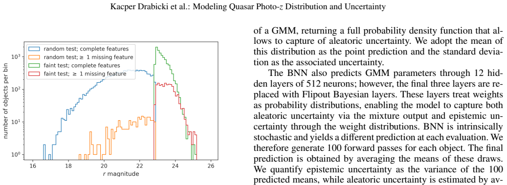
- [§2.2 and Conclusions] The ground-truth redshift distribution is the spectroscopic distribution of the DESI DR1 subsample after the SPECTYPE='QSO', ZWARN==0 cuts and the 1-arcsec cross-match. DESI target selection and redshift success are not complete or unbiased at r>22.9 or for missing-band objects. The Conclusions appropriately note that the study is an upper bound because it does not probe training-inference domain mismatch, but the body repeatedly calls this the "true" redshift distribution. All n(z) claims should be qualified as applying to the DESI-matched spectroscopic sample; otherwise the abstract's strong statement about "fundamentally unattainable" reconstruction overreaches.
minor comments (4)
- [§4.1] "The BNN achieves the lowest NLL in all three tests" is imprecise: BNN is not the lowest on the random complete test (MDN3 has -0.69 vs BNN3 -0.62). It should read "in the three tests involving additional sources of uncertainty" or similar.
- [Title/Abstract] The arXiv title and the internal manuscript title differ, and the two abstract versions are materially different (one mentions SOM/PIT, the other does not). These should be reconciled before submission.
- [§3.4] Selecting the realization with the lowest validation loss from five training runs is a form of model selection; the manuscript should state explicitly whether this selection is applied independently for each test set or only on the validation set, and whether the reported NLL values are from that single realization.
- [§4.3] The text says clusters 8 and -1 show degeneracy, and cluster -1 "usually represents outliers." Please define the cluster numbering convention and the criterion used to label a cluster as "suspicious" before reporting the 0.5%/0.2% fractions.
Circularity Check
No significant circularity: evaluation is anchored to external DESI spec-z ground truth on held-out sets; self-citations are contextual, not load-bearing.
full rationale
The paper's central comparison is empirical rather than definitional. All models are trained on KiDS-DR5 photometry with DESI-DR1 spectroscopic redshift labels and evaluated on held-out random and faint-extrapolation test sets, including missing-band subsets. The NLL, PIT, point-estimate metrics, MSE* distribution comparisons, and clustering diagnostics are all computed against external spectroscopic redshifts, so the reported rankings are not constructed from the quantities being predicted. The only flagged problem in the manuscript is an internal consistency issue: the Abstract states that 'in the hardest faint-plus-missing regime the single Gaussian becomes the best-calibrated,' whereas Table 2 gives MDN 1 an NLL of 1.28 in that regime versus 0.69 for BNN 3, i.e., the single Gaussian has the worst NLL by that metric. This is a correctness/consistency concern, not a circularity concern, and it does not make the derivation equivalent to its inputs. The paper's own limitation that it is an 'upper bound' because it 'does not explicitly probe the additional effects of training–inference domain mismatch' further limits external generalization but is also not circular. Self-citations (e.g., Nakoneczny et al. 2021, Bilicki et al. 2021) are used for data-product context and prior KiDS photo-z work, not as the load-bearing justification for the present model ranking. No fitted parameter is renamed as a prediction, no uniqueness theorem is imported from the authors' prior work, and no ansatz is smuggled in via self-citation. The derivation is therefore self-contained with respect to its external ground truth.
Axiom & Free-Parameter Ledger
free parameters (13)
- ANN architecture =
11 hidden layers x 256 neurons
- MDN/BNN architecture =
12 hidden layers x 512 neurons
- Dropout rate =
0.2
- Learning rate =
1e-4
- Early stopping patience =
30 epochs
- Model selection across training runs =
5 runs, best validation loss
- Number of GMM components =
1-5, with k=3 recommended
- Missing magnitude imputation =
maximum feature value in training subset
- t-SNE perplexity / learning rate =
40 / 200
- HDBSCAN min_cluster_size / min_samples =
50 / 5
- n(z) bin width and Monte Carlo draws =
delta_z=0.3, 5000 draws
- BNN forward passes =
100
- MSE* normalization factor =
10^3
axioms (7)
- domain assumption Spectroscopic redshifts from DESI DR1 are accurate and unbiased for matched quasars.
- domain assumption Cross-match within 1 arcsec correctly identifies the same quasar in KiDS and DESI.
- ad hoc to paper Imputing missing features with the training-set maximum preserves the test distribution for evaluating missing-band robustness.
- domain assumption ANN/MDN/BNN training with NLL/MSE losses and early stopping yields converged, representative models.
- domain assumption The 'top 10% r>22.9' subset constitutes out-of-distribution extrapolation.
- domain assumption Mean of the predicted PDF is the appropriate point estimator.
- domain assumption Adding magnitude errors as features would not improve performance.
Cite this review
Pith. "Pith review of Quasar photometric redshifts beyond the spectroscopic coverage: Uncertainty models and redshift distributions in the Kilo-Degree Survey DR5." pith.science (2026). https://pith.science/paper/SAZ7SYPJ
@misc{pith2026260319882,
  author       = {Pith},
  title        = {Pith review of: Quasar photometric redshifts beyond the spectroscopic coverage: Uncertainty models and redshift distributions in the Kilo-Degree Survey DR5},
  year         = {2026},
  howpublished = {\url{https://pith.science/paper/SAZ7SYPJ}},
  note         = {Machine review of arXiv:2603.19882}
}
abstract
Photometric redshifts (photo-$z$) and their distributions underpin cosmology with photometric quasars, tracers in angular clustering and cross-correlations. Progress requires trustworthy uncertainties, especially beyond the spectroscopic training set. We compare how machine-learning frameworks estimate quasar photo-$z$ uncertainties and reconstruct the redshift distribution $n(z)$ under controlled data-quality shifts. Using Kilo-Degree Survey DR5 photometry and DESI DR1 spectroscopic quasars, we train artificial neural networks (ANNs), Mixture Density Networks (MDNs) and Bayesian Neural Networks (BNNs) with Gaussian-mixture outputs, plus a self-organizing map (SOM) as a direct $n(z)$ estimator. We evaluate them on four subsets, with and without magnitude extrapolation and missing bands, through the negative log-likelihood, probability integral transform, point-estimate accuracy and the bias of binned $n(z)$ moments; degeneracies are sought by clustering the predicted PDFs. At least two mixture components are essential: a single Gaussian is miscalibrated and produces more catastrophic outliers than the ANN. No model performs best everywhere. On well-covered data the five-component MDN, three-component BNN and SOM reconstruct $n(z)$ almost perfectly; under faint extrapolation the BNN gives the best likelihoods, while in the hardest faint-plus-missing regime the single Gaussian becomes the best-calibrated. For point estimates and tomographic binning, uncertainty models outperform the ANN, while the SOM fails out-of-distribution. PDF clustering exposes distinct colour-redshift degeneracies likely to grow for fainter samples. The best model is thus regime- and application-dependent: multi-component MDNs or BNNs are needed for clean binning and are the only intrinsically calibrated choice on a well-covered golden sample, a first step towards a full comparison of quasar photo-$z$ pipelines.
Figures


Reference graph
Works this paper leans on
-
[1]
2015, TensorFlow: Large-Scale Ma- chine Learning on Heterogeneous Systems, software available from tensor- flow.org
Abadi, M., Agarwal, A., Barham, P., et al. 2015, TensorFlow: Large-Scale Ma- chine Learning on Heterogeneous Systems, software available from tensor- flow.org
2015
-
[2]
J., & Schwarz, D
Alonso, D., Bellini, E., Hale, C., Jarvis, M. J., & Schwarz, D. J. 2021, MNRAS, 502, 876
2021
-
[3]
2021, A&A, 653, A82
Bilicki, M., Dvornik, A., Hoekstra, H., et al. 2021, A&A, 653, A82
2021
-
[4]
2025, arXiv e-prints, arXiv:2512.16010
Chen, J., Luo, Z., Fu, L., et al. 2025, arXiv e-prints, arXiv:2512.16010
arXiv 2025
-
[5]
2015, keras,https://github.com/fchollet/keras da Costa-Luis, C
Chollet, F. 2015, keras,https://github.com/fchollet/keras da Costa-Luis, C. 2019, The Journal of Open Source Software, 4, 1277 DESI Collaboration, Aghamousa, A., Aguilar, J., et al. 2016, arXiv e-prints, arXiv:1611.00036 DESI Collaboration, Karim, M. A., Adame, A. G., et al. 2025, arXiv e-prints, arXiv:2503.14745 D’Isanto, A. & Polsterer, K. L. 2018, A&A,...
Pith/arXiv arXiv 2015
-
[6]
2013, The Messenger, 154, 32
Edge, A., Sutherland, W., Kuijken, K., et al. 2013, The Messenger, 154, 32
2013
-
[7]
M., Shanks, T., Metcalfe, N., et al
Eltvedt, A. M., Shanks, T., Metcalfe, N., et al. 2024, MNRAS, 535, 2105 Euclid Collaboration, Scaramella, R., Amiaux, J., et al. 2022, A&A, 662, A112
2024
-
[8]
2012, arXiv e-prints, arXiv:1208.4012
Green, J., Schechter, P., Baltay, C., et al. 2012, arXiv e-prints, arXiv:1208.4012
Pith/arXiv arXiv 2012
-
[9]
R., Millman, K
Harris, C. R., Millman, K. J., van der Walt, S. J., et al. 2020, Nature, 585, 357
2020
-
[10]
2010, A&A, 523, A31
Hildebrandt, H., Arnouts, S., Capak, P., et al. 2010, A&A, 523, A31
2010
-
[11]
L., Wright, A
Hildebrandt, H., van den Busch, J. L., Wright, A. H., et al. 2021, A&A, 647, A124
2021
-
[12]
Hunter, J. D. 2007, Computing in Science & Engineering, 9, 90 Ivezi´c, Ž., Kahn, S. M., Tyson, J. A., et al. 2019, ApJ, 873, 111 John William, A., Bilicki, M., Hellwing, W. A., Nakoneczny, S. J., & Jalan, P. 2025a, arXiv e-prints, arXiv:2511.17311 John William, A., Jalan, P., Bilicki, M., et al. 2025b, A&A, 698, A276
arXiv 2007
-
[13]
2024, ApJ, 964, 130
Jones, E., Do, T., Boscoe, B., et al. 2024, ApJ, 964, 130
2024
-
[14]
Kingma, D. P. & Ba, J. 2014, arXiv preprint arXiv:1412.6980
Pith/arXiv arXiv 2014
-
[15]
2008, A&A, 482, 1053
Kuijken, K. 2008, A&A, 482, 1053
2008
-
[16]
2019, A&A, 625, A2
Kuijken, K., Heymans, C., Dvornik, A., et al. 2019, A&A, 625, A2
2019
-
[17]
2015, MNRAS, 454, 3500
Kuijken, K., Heymans, C., Hildebrandt, H., et al. 2015, MNRAS, 454, 3500
2015
-
[18]
R., Feng, H., et al
Li, R., Napolitano, N. R., Feng, H., et al. 2022, A&A, 666, A85
2022
-
[19]
2024, MNRAS, 535, 1844
Luo, Z., Li, Y ., Lu, J., et al. 2024, MNRAS, 535, 1844
2024
-
[20]
2017, Journal of Open Source Software, 2, 205
McInnes, L., Healy, J., & Astels, S. 2017, Journal of Open Source Software, 2, 205
2017
-
[21]
J., Alonso, D., Bilicki, M., et al
Nakoneczny, S. J., Alonso, D., Bilicki, M., et al. 2024, A&A, 681, A105
2024
-
[22]
J., Bilicki, M., Pollo, A., et al
Nakoneczny, S. J., Bilicki, M., Pollo, A., et al. 2021, A&A, 649, A81
2021
-
[23]
Newman, J. A. & Gruen, D. 2022, ARA&A, 60, 363
2022
-
[24]
2019, A&A, 621, A26
Pasquet, J., Bertin, E., Treyer, M., Arnouts, S., & Fouchez, D. 2019, A&A, 621, A26
2019
-
[25]
2011, Journal of Machine Learning Research, 12, 2825 Pérez, F
Pedregosa, F., Varoquaux, G., Gramfort, A., et al. 2011, Journal of Machine Learning Research, 12, 2825 Pérez, F. & Granger, B. E. 2007, Computing in Science and Engineering, 9, 21
2011
-
[26]
C., Hickox, R
Petter, G. C., Hickox, R. C., Alexander, D. M., et al. 2023, ApJ, 946, 27
2023
-
[27]
2019, Nature Astronomy, 3, 212
Salvato, M., Ilbert, O., & Hoyle, B. 2019, Nature Astronomy, 3, 212
2019
-
[28]
2023, A&A, 675, A202 van der Maaten, L
Vakili, M., Hoekstra, H., Bilicki, M., et al. 2023, A&A, 675, A202 van der Maaten, L. & Hinton, G. 2008, Journal of Machine Learning Research, 9, 2579 Van Rossum, G. & Drake, F. L. 2009, Python 3 Reference Manual (Scotts Valley, CA: CreateSpace)
2023
-
[29]
E., et al
Virtanen, P., Gommers, R., Oliphant, T. E., et al. 2020, Nature Methods, 17, 261
2020
-
[30]
Waskom, M. L. 2021, Journal of Open Source Software, 6, 3021 Wes McKinney. 2010, in Proceedings of the 9th Python in Science Conference, ed. Stéfan van der Walt & Jarrod Millman, 56 – 61
2021
-
[31]
H., Kuijken, K., Hildebrandt, H., et al
Wright, A. H., Kuijken, K., Hildebrandt, H., et al. 2024, A&A, 686, A170
2024
-
[32]
2024, AJ, 168, 244
Zhang, C., Wang, W., Qu, M., Jiang, B., & Zhang, Y . 2024, AJ, 168, 244
2024
-
[33]
2022, Research in Astronomy and As- trophysics, 22, 115017 Article number, page 8 Kacper Drabicki et al.: Modeling Quasar Photo-zDistribution and Uncertainty Fig
Zhou, X., Gong, Y ., Meng, X.-M., et al. 2022, Research in Astronomy and As- trophysics, 22, 115017 Article number, page 8 Kacper Drabicki et al.: Modeling Quasar Photo-zDistribution and Uncertainty Fig. 4.Spectroscopic and photometric redshift distributions for all clusters. Article number, page 9
2022
This paper was first reviewed by deepseek-v4-flash on August 4, 2026.
discussion (0)
Sign in with ORCID, Apple, or X to comment. Anyone can read and Pith papers without signing in.