REVIEW 2 major objections 4 minor 15 references
Temperature chaos in directed polymers
T0 review · 2 major / 4 minor · reviewed 2026-08-01 · deepseek-v4-flash
Pith's one-line read The paper proves that in a canonical random polymer model, free energies at two inverse temperatures become independent directed landscapes when the temperatures are far apart.
desk verdict Genuinely new decoupling theorem and black-noise proof, with a repairable L2 gap in the independence argument and a load-bearing influence bound I could not fully verify in the visible text. read the letter →
The pith
A machine-rendered reading of the paper's core claim, the machinery that carries it, and where it could break.
The reading
What carries the argument
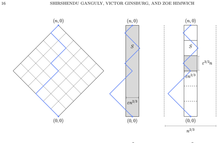
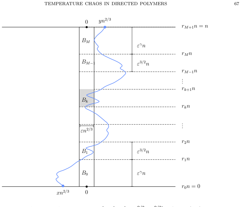
The central mechanism is the thin-strip influence bound. For a spatial strip S of half-width epsilon beta2^{2/3}, the L2 sensitivity of the beta2 free energy to resampling the white noise inside S is at most epsilon^alpha for small epsilon. This is proved via an Efron–Stein inequality for white noise: the strip is tiled into boxes and the total influence is bounded by the sum of per-box influences. Each per-box influence is small because the polymer crosses a given small box with probability about the box's width in transversal units, and when it does, the energy change is controlled by the KPZ fluctuation on that box's scale. Brownian comparison estimates for the Airy line ensemble (or its
What would settle it
Simulate two coupled CDRP free-energy profiles H_beta1 and H_beta2 with beta1=o(beta2), and measure the covariance of their finite-dimensional distributions; if the covariance does not vanish as beta2/beta1 →∞, Theorem 1.7 is false. A sharper check targets the localization input: measure the quenched transversal fluctuation exponent of the CDRP polymer at large beta; if the typical width is not of order beta^{2/3}, the strip argument fails.
Extended reading notes
Core claim
Coupled through the same space-time white noise, the CDRP free energy profiles H_beta1 and H_beta2, scaled to their natural KPZ units, converge in distribution as beta1,beta2 →∞ with beta1=o(beta2) to (L1,L2), where L1 and L2 are independent directed landscapes. The theorem is proved by showing that the beta1-polymer is localized inside a thin spatial strip of width of order beta2^{2/3} around its typical path, that the beta1 free energy is nearly measurable with respect to the noise in that strip, and that resampling the noise inside any such thin strip changes the beta2 free energy negligibly. Thus the two free-energy profiles become functions of essentially independent pieces of the noise
Load-bearing premise
The argument stands on the CDRP polymer localization estimate imported from an earlier work: at inverse temperature beta and over a unit time interval, the polymer's transversal displacement has typical scale beta^{2/3} with stretched-exponential tails. If this scale is not exactly beta^{2/3}, the strip either fails to contain the beta1 polymer or the decoupling regime beta1=o(beta2) is not the correct one.
Editorial extensions
If this is right
- If Theorem 1.7 holds, temperature chaos is rigorous in the CDRP: the free-energy profiles at well-separated temperatures are asymptotically independent, not merely decorrelated.
- The same machinery proves the directed landscape is a two-dimensional black noise, making it the third known example after critical planar percolation and the Brownian web.
- Polymer measures at any two distinct inverse temperatures are mutually singular almost surely, even when free energies are strongly correlated; the path-space Gibbs measures live on different energy-level sets.
- For temperatures that are polynomially close, the coupled pair converges to two copies of the same directed landscape, so the chaos transition must occur at a nontrivial separation scale.
- A sharp threshold is conjectured at beta2 - beta1 ~ beta1^{1/3}; the paper proves stability and decoupling on either side of that scale but leaves the threshold itself open.
Reading between the lines
- One plausible extension is that the same thin-strip mechanism transfers from the CDRP to discrete lattice directed polymers in the strong-disorder regime, predicting the experimentally relevant n^{-1/6} temperature-perturbation scale; the paper only sketches this connection.
- If the directed landscape is a two-dimensional black noise, then any finite-resolution white-noise approximation of the landscape sees it only through high-frequency components, a feature that could matter for numerical simulations of interface growth.
- The same influence method may show that the critical two-dimensional stochastic heat flow is a three-dimensional black noise, which would be the first known example in dimension three or higher.
- The relation between temperature and disorder chaos sketched in the paper suggests a testable equivalence: the critical temperature-perturbation scale should match the disorder-perturbation scale under a reparameterization, a prediction that finite-size simulations could probe.
Editorial analysis
A structured set of objections, weighed in public.
Referee Report
Summary. The manuscript studies temperature chaos for the continuum directed random polymer (CDRP). Its central result, Theorem 1.7, states that when two CDRP free-energy profiles at inverse temperatures β1 and β2 are coupled through the same white noise and β1,β2→∞ with β1=o(β2), the pair converges in distribution to two independent directed landscapes. The proof is built on a thin-strip influence bound (Theorem 5.2), proved via a white-noise version of the Efron–Stein inequality, together with imported convergence and localization results for the CDRP and the directed landscape. As a byproduct, the authors prove that the directed landscape is a two-dimensional black noise (Theorem 1.9), resolving a conjecture of Virág. They also prove mutual singularity of CDRP polymer measures at different temperatures and formulate a conjecture for the sharp temperature-chaos exponent.
Significance. If completed, this would be the first rigorous energetic temperature-chaos result for a canonical KPZ-universality model, with the limiting pair explicitly identified as independent copies of the universal zero-temperature object. The measure-theoretic framework for restricted CDRP partition functions and the influence estimates are likely to be reusable. The black-noise theorem resolves an open conjecture and provides a third known example of a two-dimensional black noise. The paper is unusually careful about measurability and resampling of white noise, and the overall proof architecture is coherent and detailed.
major comments (2)
- [§5, proof of Theorem 1.7 / Lemma 5.4] Lemma 5.4 is invoked with X_n=Hbar^ξ_{β1}(u), Z_n=Hbar^ξ_{β1,S}(u), but the lemma requires limsup E||X_n−Z_n||^2 ≤ ε. Lemma 5.1 only establishes convergence in probability. Proposition 4.14 controls the quenched probability of polymer exit on a high-probability event, but it does not, as stated, control the size of |log p| on the exceptional event where the exit probability is not small. An additional integrability statement for the restricted free energy, or a modification of Lemma 5.4 requiring only convergence in probability, is needed. As written, the independence conclusion does not formally follow from the stated lemmas.
- [§5, proof of Theorem 1.7] There is a second formal mismatch with Lemma 5.4. The lemma requires ||Y_n−W_n||_p → 0 for the sequences associated with each ε>0. Theorem 5.2 gives only limsup E|Hbar^ξ_{β2}−Hbar^{η_S}_{β2}|^2 ≤ ε^α for a fixed ε>0. Since ε is fixed in the application, this bound does not vanish. To obtain the desired tensorization one must either diagonalize over ε→0 or state a variant of Lemma 5.4 in which both approximation errors satisfy limsup ≤ ε. The current proof does not supply this step, leaving the central claim incomplete.
minor comments (4)
- [§5, Eq. (5.3)] The notation H^ξ_{β1,S} for the restricted free energy is very close to H^ξ_{β1}; consider a different symbol (e.g., H^{ξ,strip}_{β1}) to avoid confusion in a long proof.
- [§5, Lemma 5.1] The endpoint scaling in the strip uses factors 2^{1/3}β^{2/3}; it would help to state explicitly how these factors are absorbed by the constants in Proposition 4.14 and the convergence in Theorem 1.5.
- [§1.5 / §7.9] Section 7.9 is a sketch of a possible SHF result rather than a theorem. This is acceptable, but it should be labeled more prominently as heuristic/sketch so that it is not read as a claim.
- [References] Some citations, e.g., [QR V25], contain a space in the author field. Please check the reference formatting.
Circularity Check
No significant circularity: the decoupling theorem follows from external convergence/localization inputs and a new influence estimate; self-citations are background only.
full rationale
The derivation of Theorem 1.7 does not reduce to its own inputs. Marginal convergence to the directed landscape is an external input ([Wu26, Theorem 1.6], stated as Theorem 1.5); the polymer localization entering Lemma 5.1 is [DZ24, Corollary 3.5] (Proposition 4.14); and the new thin-strip influence bound (Theorem 5.2) is proved in Section 6 from the Efron–Stein inequality for white noise together with those external scaling and regularity estimates. The restricted free energy H_{β1,S} is not defined in terms of H_{β2}; the approximation H_{β1,S} ≈ H_{β1} is a consequence of the external localization estimate in the regime β1 = o(β2), not an identity imposed by construction. The independence of the approximating vectors in Lemma 5.4 comes from Proposition 2.2 (measurability of the restricted free energy) and the independent-resampling coupling, not from assuming the conclusion. Theorem 1.9 is proved through a separate discrete LPP proxy (Sections 7.5–7.6), not by assuming Theorem 1.7. The only caveat is a written-proof gap: Lemma 5.1 establishes convergence in probability for the restricted-energy difference, while Lemma 5.4 asks for an L^2 bound; this is likely repairable from the uniform fourth-moment bound (Lemma 4.5) plus localization tails, but it is a completeness/correctness issue, not circularity. Self-citations such as [GH24a, GH23a] and [GG] appear only in background or outlook and are not load-bearing.
Assumptions & free parameters
free parameters (2)
- alpha (influence exponent, Theorem 5.2 / Theorem 6.1) =
unspecified; only existence of some alpha > 0 is claimed (Remark 5.3: true order expected epsilon^{1/2})
- gamma (mesh boundary exponent, Section 6.2) =
any value in (0, 1/6)
assumptions (9)
- domain assumption [AJRAS22, Theorem 2.2]: existence and regularity of the CDRP partition function process Z^xi_beta(s,x;t,y) with chaos expansion (3.16), strict positivity, Chapman–Kolmogorov (Theorem 3.12 here)
- domain assumption [Wu26, Theorem 1.6]: zero-temperature convergence of the CDRP free energy profile to the directed landscape (Theorem 1.5 here)
- domain assumption [DZ24, Corollary 3.5 and Theorem 1.10]: polymer transversal fluctuation bounds and annealed polymer convergence to the directed landscape geodesic (Propositions 4.14, 4.15)
- domain assumption [CHH23, Theorem 1.1]: local Brownianity of parabolic Airy/KPZ line ensembles (Proposition 4.6)
- domain assumption [DOV22] and [GZ22, Lemma 3.11]: construction and regularity of the directed landscape (metric composition, scaling, Holder continuity, geodesic transversal fluctuations), Propositions 4.1–4.3, 4.12–4.13
- domain assumption [CG20a, CG20b]: stretched-exponential upper/lower tail bounds for the CDRP free energy (Lemma 4.5)
- domain assumption [HP24]: the directed landscape is a one-dimensional black noise in the time direction
- domain assumption [QRV25]: Gaussian multiplicative chaos framework for CDRP (used in Section 8)
- standard math Standard Gaussian analysis and measure theory: Wiener chaos expansion, martingale convergence, Efron–Stein inequality on product spaces, Doob–Dynkin factorization (Section 3)
invented entities (1)
-
Restricted length L_R and sigma-algebras F_R of the directed landscape
independent evidence
Cite this review
Pith. "Pith review of Temperature chaos in directed polymers." pith.science (2026). https://pith.science/paper/SI5Q7XPS
@misc{pith2026260718194,
  author       = {Pith},
  title        = {Pith review of: Temperature chaos in directed polymers},
  year         = {2026},
  howpublished = {\url{https://pith.science/paper/SI5Q7XPS}},
  note         = {Machine review of arXiv:2607.18194}
}
abstract
Disordered systems such as spin glasses and polymers characteristically exhibit random energy landscapes with many macroscopically separated energetic valleys corresponding to near-ground states. This high complexity renders these systems extremely sensitive to perturbations of external parameters. For instance, the support of associated Gibbs measures may change macroscopically under such perturbations, a phenomenon known as chaos in the literature. In experiments, chaotic phenomena are typically studied via temperature perturbations. In this article, we initiate the rigorous study of temperature-chaotic properties of the continuum directed random polymer (CDRP), a canonical model in the KPZ universality class. The CDRP is driven by white noise and is parametrized by inverse temperature $\beta$, and is known [Wu '26, Das-Zhu '24] to converge in the zero-temperature limit $\beta \to \infty$ to the directed landscape constructed in [Dauvergne-Ortmann-Vir\'ag '22], the putative universal scaling limit of models in the KPZ universality class. The main result of this article considers the CDRP free energies coupled through the same white noise at a pair of inverse temperatures $(\beta_1, \beta_2)$, and shows that they decouple in the limit $\beta_2 \gg \beta_1 \gg 1$, converging to a pair of independent directed landscapes. This is the first such "energetic de-correlation across temperatures" result. Our key estimate measures the "pivotality" or "influence" of spatially thin strips in models of last passage percolation. As a byproduct, the proof strategy also allows to show that the directed landscape is a two-dimensional black noise (in the sense of [Tsirelson-Vershik '98]), previously conjectured by Vir\'ag. This provides the third known example of a two-dimensional black noise after critical planar percolation [Schramm-Smirnov '11] and the Brownian web [Ellis-Feldheim '16].
Figures


Figures from the paper (14 more)




Reference graph
Works this paper leans on
-
[7]
[CD25] Francesco Caravenna and Anna Donadini. Enhanced noise sensitivity, 2D directed polymers and stochas- tic heat flow.arXiv preprint arXiv:2507.10379,
-
[8]
[COTX26] Le Chen, Cheng Ouyang, Samy Tindel, and Panqiu Xia. A class of d-dimensional directed polymers in a Gaussian environment.arXiv preprint arXiv:2603.06574,
-
[11]
[GZ22] Shirshendu Ganguly and Lingfu Zhang. Fractal geometry of the space-time difference profile in the directed landscape via construction of geodesic local times.arXiv preprint arXiv:2204.01674,
-
[13]
Introduction to KPZ
[Qua12] Jeremy Quastel. Introduction to KPZ. InCurrent developments in mathematics, 2011, pages 125–194. Int. Press, Somerville, MA,
2011
-
[1963]
The heat and the landscape I.arXiv preprint arXiv:2008.07241,
[Vir20] B´ alint Vir´ ag. The heat and the landscape I.arXiv preprint arXiv:2008.07241,
arXiv 2008
-
[1996]
[BSS14] Riddhipratim Basu, Vladas Sidoravicius, and Allan Sly. Last passage percolation with a defect line and the solution of the slow bond problem.arXiv preprint arXiv:1408.3464,
-
[2006]
Unabridged republication of the 1967 original. [Tsa24] Li-Cheng Tsai. Stochastic heat flow by moments.arXiv preprint arXiv:2410.14657,
arXiv 1967
-
[2010]
The directed landscape is a black noise.arXiv preprint arXiv:2404.16801,
[HP24] Zoe Himwich and Shalin Parekh. The directed landscape is a black noise.arXiv preprint arXiv:2404.16801,
Show all 15 references
-
[2014]
Rotationally invariant first passage percolation: Concentration and scaling relations.arXiv preprint arXiv:2312.14143,
[BSS23] Riddhipratim Basu, Vladas Sidoravicius, and Allan Sly. Rotationally invariant first passage percolation: Concentration and scaling relations.arXiv preprint arXiv:2312.14143,
-
[2015]
Stochastic heat flow is a black noise.arXiv preprint arXiv:2506.16484,
[GT25] Yu Gu and Li-Cheng Tsai. Stochastic heat flow is a black noise.arXiv preprint arXiv:2506.16484,
-
[2019]
Geometry of the Gaussian multiplicative chaos in the Wiener space.arXiv preprint arXiv:2008.04290,
[BM20] Yannic Br¨ oker and Chiranjib Mukherjee. Geometry of the Gaussian multiplicative chaos in the Wiener space.arXiv preprint arXiv:2008.04290,
2008 arXiv
-
[2021]
The scaling limit of the longest increasing subsequence.arXiv preprint arXiv:2104.08210,
[DV21] Duncan Dauvergne and B´ alint Vir´ ag. The scaling limit of the longest increasing subsequence.arXiv preprint arXiv:2104.08210,
-
[2024]
Geodesic switches and exceptional times in dynamical Brownian last passage percolation
[Bha25a] Manan Bhatia. Geodesic switches and exceptional times in dynamical Brownian last passage percolation. arXiv preprint arXiv:2510.27589,
-
[2025]
Near-existence of bigeodesics in dynamical exponential last passage percolation.arXiv preprint arXiv:2504.12293,
[Bha25b] Manan Bhatia. Near-existence of bigeodesics in dynamical exponential last passage percolation.arXiv preprint arXiv:2504.12293,
-
[2026]
The Green’s function of the parabolic Anderson model and the continuum directed polymer.arXiv preprint arXiv:2208.11255,
[AJRAS22] Tom Alberts, Christopher Janjigian, Firas Rassoul-Agha, and Timo Sepp¨ al¨ ainen. The Green’s function of the parabolic Anderson model and the continuum directed polymer.arXiv preprint arXiv:2208.11255,
Reviewed August 1, 2026 · model on record in the stance chip above.
Discussion (0). Continue with ORCID to comment.