Dubrovin-Natanzon divisors on MM-curves

Petr G. Grinevich; Simonetta Abenda

REVIEW 4 major objections 5 minor 47 references

Dubrovin-Natanzon divisors on MM-curves

T0 review · 4 major / 5 minor · reviewed 2026-08-05 · deepseek-v4-flash

Challenge this review Re-run · record.json Download PDF Read on arXiv ↗

Pith's one-line read On MM-curves from totally positive Schubert cells, every non-smooth DN divisor is a combination of two elementary blow-ups.

desk verdict New classification of non-smooth DN divisors on Schubert-cell MM-curves, but the proof leans on an unproved perturbation step that needs to be made rigorous. read the letter →

arxiv 2508.08426 v1 pith:SQEVZKTL submitted 2025-08-11 math.AG math-phmath.COmath.MPnlin.SI

Simonetta Abenda , Petr G. Grinevich This is my paper · ORCID

classification math.AGmath-phmath.COmath.MPnlin.SI MSC 14H7014T2037K10

keywords MM-curvesDubrovin-NatanzondivisorsKPIIequationtotallynonnegativeGrassmannianspositroidcellsLe-graphsblow-upsrealregularsolitons

verification ladder T0 review T1 audit T2 compute T3 formal

The pith

A machine-rendered reading of the paper's core claim, the machinery that carries it, and where it could break.

The reading

The paper closes a gap in the bridge between soliton theory and algebraic geometry: real regular KP II solutions correspond to Dubrovin-Natanzon (DN) divisors on M-curves, but on the rational limiting curves called MM-curves (maximal Mumford curves, the rational degenerations that keep $g+1$ real ovals) the divisor can become non-smooth, and earlier constructions avoided this by choosing a special normalization time. To parameterize a whole positroid cell by divisors one must fix the time and understand the non-smooth events. The paper proves that for MM-curves dual to Le-graphs of totally positive Schubert cells — positroid cells whose Young diagram is completely filled — only two local degenerations can occur: two divisor points meeting at a double point, or three divisor points meeting at a trivalent black vertex. Each is resolved by a standard blow-up, and every non-smooth DN divisor is a combination of these two. The exclusion of all other configurations rests on a counting argument that compares marked white vertices with the faces of the marked region on the Le-graph.

What carries the argument

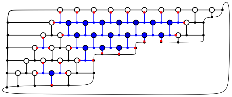
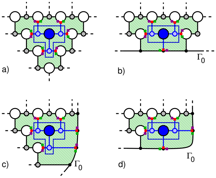
The load-bearing machinery is the DN condition on an MM-curve together with a marking game on its Le-graph. On white-vertex components the wave function is a degree-one rational function; on black-vertex components it is constant. Mark every vertex whose component makes the wave function vanish identically, mark adjacent edges, and place a red divisor point at each edge joining a marked component to an unmarked one. Lemma 3 says components touching the infinite oval can never be marked, because the DN condition forces strict positivity there. The key count (Corollary 1) is that any connected marked region has fewer internal faces than marked white vertices; with one divisor point per face th

What would settle it

A concrete counterexample: an MM-curve dual to the Le-graph of a totally positive Schubert cell and a time $\vec{t}$ at which a DN divisor has a non-smooth configuration other than the two allowed types — e.g., three divisor points meeting at a double point on a white/$\Gamma_0$ edge, or two divisor points meeting at a trivalent black vertex — while the Abel transform stays finite. Alternatively, a purely combinatorial falsifier is a connected marked region in such a Le-graph, consistent with Lemmas 1–3, whose internal faces are at least as numerous as its marked white vertices, which would br

Watch

Extended reading notes

Core claim

Main result (Theorem 1): let $\Gamma$ be an MM-curve dual to the Le-graph of a totally positive Schubert cell, and let $D$ satisfy the Dubrovin-Natanzon conditions — one divisor point on each finite real oval, and $\operatorname{Im} A_l(D) = \pi \pmod{2\pi}$ for every basic cycle $l$. Then (1) for any times $\vec{t}$, the Krichever wave function does not vanish identically on any $\mathbb{CP}^1$ component of a white vertex; (2) the only non-smooth divisor configurations are the two basic types: two divisor points meeting at the two ends of a white/$\Gamma_0$ edge, and three divisor points meeting at the three ends of a trivalent black vertex. These are resolved by blow-ups (14) and (15); hen

Load-bearing premise

The counting proof of Part 1 assumes that a small generic shift of time moves every boundary ('red') divisor point continuously into the interior of a surrounding face, that each such face receives exactly one red point, and that the set of marked white vertices does not change; if a red point could cross a face boundary or a white vertex could stop being marked, the contradiction that rules out the assumed configuration would not follow.

Editorial extensions

If this is right

With a fixed normalization time, every totally positive Schubert positroid cell can be covered by DN divisor data including its boundary, since non-smooth divisors are classified by the two blow-ups.
For all KP II evolution times $\vec{t}$, the wave function never vanishes identically on a white-vertex component, so the spectral curve construction never degenerates in that way.
Checking admissibility of a singular divisor reduces to checking the finite ratios that define the blow-up coordinates in (14) and (15), instead of analyzing arbitrary collisions.
The two blow-ups give a finite local list for the boundary behavior of the Abel transform on MM-curves, usable in further degeneration limits.
This is the first step toward a full divisor parametrization of positroid cells for KP II multiline solitons with a fixed normalization time, complementing the earlier smooth construction.

Reading between the lines

Editorial extensions of the paper, not claims the author makes directly.

Our inference: Corollary 1's inequality — internal faces of a marked region are fewer than its marked white vertices — is a purely graph-theoretic statement about Le-graphs of totally positive Schubert cells; extracting and proving it separately would let the counting be verified by direct enumeration over Young diagrams.
Our inference: the blow-up ratios in (14) and (15) are natural candidates for local coordinates on the lower-dimensional strata of the positroid cell, suggesting a concrete dictionary between divisor collisions and the cell decomposition of the totally nonnegative Grassmannian.
Our inference: for non-Schubertt positroid cells or non-trivalent graphs, additional non-smooth configurations should appear; the restriction to totally positive Schubert cells (all boxes in the Young diagram filled) is likely essential rather than a technical convenience.

Share X Bluesky LinkedIn Reddit HN

Editorial analysis

A structured set of objections, weighed in public.

Desk editor's note, referee report, and a circularity audit.

Desk Editor's Note

read the letter

Colleague, the paper by Abenda and Grinevich tackles something real: for MM-curves dual to trivalent Le-graphs of totally positive Schubert cells, they claim that any non-smooth DN divisor arises via just two local blow-up models. That is genuinely new—their earlier work deliberately swept non-smooth divisors under the rug by choosing a normalization time, and here they fix the time and classify the singular limits. The two blow-ups (14) and (15) are explicit and the local Abel-transform asymptotics in Section 4 are convincing. If the theorem holds, this is a concrete step toward parametrizing the full positroid cell by spectral data.

The soft spot is the proof of Part 1. The paper omits proofs of Lemmas 1 and 4, saying they follow directly or immediately from the wave function properties. That alone would be tolerable if the core argument were airtight, but the decisive step—the one that actually uses the DN condition—is a deformation claim: a small generic perturbation of the time is said to move each red divisor point into exactly one surrounding green face, to keep the marked white vertices unchanged, and to put revived zeros only in internal faces. None of that is proved. The stress-test note is right: identically-vanishing on a white component is a special condition on t, so a generic perturbation could destroy the marking before the counting starts; a red point could cross a double point into a different face; and a revived zero could land in a surrounding face rather than an internal one. Any one of those would break the pigeonhole argument in Corollary 1. Since Part 2 is deduced from Part 1, the whole classification rests on this perturbation-continuity lemma.

Let me be clear: I don't see a fatal error, and the gap may be fillable with a careful argument using the explicit form of the wave function and the DN inequalities. But as written, the main theorem is conditional. The combinatorial structure of the marked-area propagation (Lemma 4) looks plausible and is probably correct, but it's presented as 'immediate' and deserves a full proof.

The paper is worth a serious referee. It is clearly written, the statement is precise, and the claimed dichotomy is important for the finite-gap degeneration approach to KP II solitons. The right outcome is major revision: either supply the missing deformation lemma, or weaken the theorem to cover the cases that are actually proved.

Referee Report

4 major / 5 minor

Summary. The paper studies Dubrovin-Natanzon (DN) divisors on maximal Mumford (MM) curves obtained as rational degenerations of M-curves, with dual graphs given by Le-graphs of totally positive Schubert cells. The main claim (Theorem 1) is that, under the DN condition, (1) the Krichever wave function never vanishes identically on a white CP1 component for any time vector, and (2) every non-smooth divisor configuration is generated by just two types of blow-ups, described in §4 by equations (14) and (15). The proof uses a combinatorial marking of white vertices where the wave function vanishes identically, a counting argument (Corollary 1) to derive a contradiction from the DN condition, and then a classification of double-point degenerations. The paper also recalls background on KP-II solitons, totally non-negative Grassmannians, Le-networks, and the Abel transform on MM-curves.

Significance. If established, Theorem 1 would be a meaningful step toward parametrizing full positroid cells by DN divisors with a fixed normalization time, reducing all non-smooth divisor configurations to two explicit local blow-ups. The paper connects KP soliton theory, real algebraic geometry, and tropical degenerations, and the statement is crisp and falsifiable. However, the current proof has load-bearing gaps: the central perturbation argument in the proof of Part 1 is asserted without proof, and several combinatorial lemmas on which the counting rests are either unproved or dismissed as immediate. The result is plausible and likely worth pursuing, but the manuscript does not yet provide a complete proof.

major comments (4)

[§5, proof of Part 1 (paragraph after Corollary 1)] The contradiction argument depends on an unproved small-perturbation step. The authors assert that a small generic shift of the time vector t0 moves each red divisor point into a surrounding green face, one point per face, and that all divisor points associated with the marked white vertices lie in internal faces. Three specific claims are needed: (i) the set of marked white vertices is unchanged under the perturbation; (ii) each red point lands in a distinct surrounding face; (iii) a zero that reappears on a formerly identically-vanishing white component lies in an internal face of the marked area. Claim (i) is especially delicate because identical vanishing on a CP1 component is a codimension condition in t, not an open condition, so a generic perturbation may unmark vertices before any counting is possible. Claim (iii) is also unproved: if the revived zero falls into a surrounding fac
[§5, Lemmas 1 and 4] Lemma 1 is stated without proof, and Lemma 4, which contains four configuration cases and is the basis for Corollary 1, is dismissed as following immediately from Lemmas 1–3. These facts are not evident from the degree-1 rationality of the wave function on white components alone. Whether a white component vanishes identically depends on the matching data at all adjacent double points, and Lemma 1(2) ('if at least two adjacent vertices are marked, then Γ1 is marked') requires a calculation involving the pole/zero structure at the nodes. Lemma 4's assertions about the existence and marking of vertices Γ^{i+1}_j are nontrivial combinatorial statements about Le-graph geometry. Since Corollary 1 is the counting inequality used to obtain the contradiction in Part 1, these omitted proofs are load-bearing and must be supplied.
[§5, proof of Part 2] The classification into exactly the blow-ups (14) and (15) assumes without proof that a divisor point reaching a double point on a non-identically-vanishing component produces exactly one divisor point at each adjacent component (or three divisor points at the black-vertex configuration), and that these are the only possible singularities compatible with the DN condition. This is an incidence statement about the zeros of the wave function at double points and needs a precise proof. Moreover, Remark 2 notes that several such degenerations may occur simultaneously; the theorem's conclusion that only combinations of the two basic types may occur requires a global argument, not just the local examples in §4. As written, the proof of Part 2 does not exclude other simultaneous or higher-order degenerations.
[§4 and Theorem 1] The statement of Theorem 1 assumes that a non-smooth divisor D 'satisfies the DN condition', but the paper does not give a rigorous definition of the DN condition for divisors that may lie at double points or after blow-up. Equation (11) defines an Abel transform for a restricted class of divisors, and the discussion in §4 of a finite Abel transform in singular configurations is informal. A theorem that excludes all other singular configurations needs a precise notion of admissible non-smooth divisor and of what counts as a 'configuration' after blow-up. The relevant definitions from [10, 44] should be stated explicitly, or the paper should prove that the two blow-ups are exactly the operations preserving finiteness of the Abel transform and the one-point-per-finite-oval condition.

minor comments (5)

[Abstract and §1] There are typos and stylistic issues: 'possess' is misspelled as 'posses', and the sentence 'However, to show that DN divisors parameterize the; full positroid cell' contains a stray semicolon.
[§2] The name 'Druma' in the text should be 'Dryuma' (see reference [14]).
[§4] In the first paragraph, 'considered in out paper' should read 'considered in our paper'.
[§5] The informal color terminology ('salad green', 'magenta', 'blue') is used throughout the proof. The colors are helpful in the figures, but the final text would benefit from a legend or a formal label for each color class, especially in the perturbation argument.
[§5, Lemma 3] The proof of Lemma 3 refers to 'the Krichever normalization' of the wave function. This normalization should be defined or cited explicitly, since it is used to conclude strict positivity on the infinite oval.

Circularity Check

0 steps flagged · score 0.0 of 10

No circularity: Theorem 1 is a new DN-constrained classification; the two blow-up types are candidates derived from Abel asymptotics and then proved exhaustive. The flagged weak point is an unproved perturbation-continuity step, not a circular reduction.

full rationale

I found no circular reduction in the derivation. The two blow-up types are first introduced in Section 4 as local models (eqs. (14) and (15)) based on Abel-transform asymptotics for divisor points approaching double points, and Theorem 1 in Section 5 then attempts to prove that these are the only singular configurations under the DN condition. The proof uses the previously established wave-function properties on MM-curves from the authors' earlier papers [3,5,6] and the DN divisor description; these are external published results whose assumptions do not include Theorem 1, so they are independent support rather than a self-citation chain that forces the conclusion. The paper also explicitly distinguishes the theorem's scope: Remark 3 states that the statement 'essentially uses the DN conditions' and that for more generic divisors more complicated configurations are expected, so the conclusion is not definitionally identified with the two blow-up models. The main weakness is a correctness gap in the proof of Part 1 after Corollary 1: the text asserts that 'a small generic perturbation will move these red divisor points inside green areas, and each green area contains exactly one red divisor point' and that 'all divisor points at the white vertices from the marked area shall correspond to the internal faces of the marked area.' This is an unproved perturbation-continuity premise: an infinitesimal time shift could in principle change the set of marked white vertices or move a red point across a face boundary, in which case the counting contradiction would fail. That is a missing proof step, not a circularity: the contradiction is not assumed as an input. Likewise, the omitted proofs of Lemmas 1, 2, and 4 ('The proof is omitted because it directly follows from the properties of the wave function'; 'The proof immediately follows from Lemma 1') signal terseness rather than circular dependence on the theorem. Overall, the central claim is not equivalent to its inputs by construction, so the circularity score is 0.

Assumptions & free parameters 0 free parameters · 4 assumptions · 0 invented entities

The theorem's burden is carried by prior results of the same authors [3,4,5,6] describing the KP wave function and DN divisors on MM-curves. No free parameters are fitted; the weights t_ij in Le-networks are coordinates on the positroid cell, not ad hoc constants. No new entities are postulated; the two blow-up procedures are local resolution techniques, and MM-curves and Le-graphs already exist in the cited literature.

assumptions (4)

domain assumption The KP wave function extends to the MM-curve with degree 1 on white-vertex components, constant on black-vertex components, and node values determined by linear relations on the Le-graph (from [4]).
Invoked in Lemma 1 and the proof of Part 2 of Theorem 1; taken from the authors' previous paper [4] without reproof.
domain assumption For a DN divisor on an MM-curve, the wave function in Krichever normalization is real and strictly positive on the infinite oval, so white vertices in the upper row and at the left end of each row are never marked.
Used in Lemma 3; inherited from the Dubrovin-Natanzon reality analysis in [15,16] and its adaptation to MM-curves in [3,4].
domain assumption The Abel transform of a DN divisor satisfies Im A_l(D) = π mod 2π for all l, and each finite oval contains exactly one divisor point.
Definition 1 and Section 2.0.3; this is the Dubrovin-Natanzon characterization of real regular finite-gap solutions, extended to degenerate curves in [3,4].
domain assumption The dual graph of an MM-curve associated to a totally positive Schubert cell has the row/face structure used in Lemma 4 and Corollary 1: no white vertices directly connected to the boundary in upper row or left ends, and a marked connected component has triangular shape.
This follows from the Le-graph construction in [41] and the MM-curve duality in [3,4]; it is not re-derived here.

how reviews work

0 comments

Cite this review

Pith. "Pith review of Dubrovin-Natanzon divisors on MM-curves." pith.science (2026). https://pith.science/paper/SQEVZKTL

@misc{pith2026250808426,
  author       = {Pith},
  title        = {Pith review of: Dubrovin-Natanzon divisors on MM-curves},
  year         = {2026},
  howpublished = {\url{https://pith.science/paper/SQEVZKTL}},
  note         = {Machine review of arXiv:2508.08426}
}

abstract

${\mathtt{MM}}$-curves are rational degenerations of ${\mathtt{M}}$-curves, i.e. they are maximal Mumford in the sense that they posses $g$ tropical cycles and exactly $g+1$ real ovals, where $g$ is the arithmetic genus. For rational curves the ``naive'' definition of divisors as formal sums of points requires a refinement. In the finite-gap theory of KP II equation the real regular solutions correspond to the Dubrovin-Natanzon (DN) divisors on ${\mathtt{M}}$-curves. In the case of real regular multiline KP II solitons, it was shown by the authors that for any given solution there exists a normalization time such that the spectral data are smooth DN divisor on ${\mathtt{MM}}$-curve. However, to show that DN divisors parameterize the; full positroid cell, it is necessary to fix the normalization time and consider both smooth and non-smooth divisors. In this paper we start such an investigation, and show that on ${\mathtt{MM}}$-curves whose dual graphs are trivalent Le-graphs of totally positive Schubert cells, the construction of non-smooth DN divisors requires combinations of just two basic types of blow-ups.

Figures

Figures reproduced from arXiv: 2508.08426 by the authors.

**Figure 2.** Top: we mark the faces of the Le-diagram of [PITH_FULL_IMAGE:figures/full_fig_p010_2.png] view at source ↗

**Figure 3.** A basis of b-cycles and c-cycles on Γ 2. If the cycle bk does not pass through any boundary vertex, then the restriction of ωk to Γ0 is equal to zero. 3. If the cycle bk passes through an internal vertex (black or white), the differential ωk has exactly two first-order poles, with residue 1 at the outgoing point and with residue −1 at the incoming point. 4. If the cycle passes through a boundary vertex, it has first… view at source ↗

Figures from the paper (23 more)

**Figure 4.** Figure 4: The intersection of the cycles b1 and a1 with Γ1 of [PITH_FULL_IMAGE:figures/full_fig_p013_4.png]

**Figure 5.** Figure 5: An admissible divisor on Γ 14 [PITH_FULL_IMAGE:figures/full_fig_p014_5.png]

**Figure 6.** Figure 6: ). Such situation never happens in KP dynamics. Γ4 b 6 b 7 γ 4 Γ0 Γ4 b 6 b 7 Γ0 γ 6 γ 6 6 5 1 0 1 0 1 0 6 5 1 0 1 0 1 0 Σ3 Σ2 Σ3 Σ2 [PITH_FULL_IMAGE:figures/full_fig_p015_6.png]

**Figure 7.** Figure 7: ): R 2 → R 2 × RP 1 , [PITH_FULL_IMAGE:figures/full_fig_p016_7.png]

**Figure 8.** Figure 8: 3 divisor points γ2, γ3 and γ5 simultaneously pass through a triple point. Remark 2. In the example of [PITH_FULL_IMAGE:figures/full_fig_p017_8.png]

**Figure 9.** Figure 9: Example of the Le-graph of a totally positive Schubert cell with marked vertices and edges. In the current Figure marked vertices and edges are colored blue. If an edge connects a marked component to a non-marked one, we have a divisor point (marked red) at the non-mar…

**Figure 10.** Figure 10: This Figure illustrates Lemma 2. The proof immediately follows from Lemma 1. Lemma 3. The white vertices in the upper row of the diagram and the white vertices located at the left end of each row are never marked. Proof of Lemma 3. 19 [PITH_FULL_IMAGE:figures/full_fi…

**Figure 11.** Figure 11: The infinite oval is painted magenta. At the points marked ma [PITH_FULL_IMAGE:figures/full_fig_p020_11.png]

**Figure 12.** Figure 12: The faces surrounding the marked area are colored salad [PITH_FULL_IMAGE:figures/full_fig_p020_12.png]

**Figure 12.** Figure 12: This Figure illustrate the case of one isolated marked white vertex. This vertex and the black vertices adjacent to this white one are marked blue and enclosed by a blue polygon. The faces surrounding this marked area are colored salad green. For generic time ⃗t0 no d…

**Figure 13.** Figure 13: This Figure illustrates Lemma 4 case 1. Internal faces of the marked area between the rows i and i + 1 are marked blue. Γ i r is not the last white vertex in the row i. 22 [PITH_FULL_IMAGE:figures/full_fig_p022_13.png]

**Figure 14.** Figure 14: This Figure illustrates Lemma 4 case 1. Internal faces of the marked area between the rows i and i + 1 are marked blue. Γ i r is the last white vertex in the row i. 2. Let Γ i s be the first vertex directly connected to the boundary, and s > 2 then: (a) The white vert…

**Figure 15.** Figure 15: This Figure illustrates Lemma 4 case 2. Internal faces of the marked area between the rows i and i + 1 are marked blue. Γ i s is the first white vertex in the row i directly connected to the boundary. 3. Let Γ i 2 be the first vertex directly connected to the boundary…

**Figure 16.** Figure 16: This Figure illustrates Lemma 4 case 3. Γ i 2 is the first white vertex in the row i directly connected to the boundary. No faces between the rows i and i + 1 are marked. 4. If Γ i 1 is directly connected to boundary, there are no marked components in the row i + 1 b…

**Figure 17.** Figure 17: This Figure illustrates Lemma 4 case 4. The proof of Lemma 4 follows immediately from Lemmas 1-3. From Lemma 4 it immediately follows: Corollary 1. 1. The number of internal faces in a connected marked area between lines i and i + 1 is equal to the number of marked wh…

**Figure 18.** Figure 18: One connected component of the marked region is enclosed by a blue polygon. The faces surrounding this marked area are colored salad green. Internal faces of the marked area are colored blue. To prove Part 2, let us remark the following. First of all, two components c…

**Figure 19.** Figure 19: On the left: A matrix representing a point in Gr(4, 10) written in reduced row echelon form. On the right: the corresponding Young diagram (English notation). Pivot columns are 1, 3, 6, 8; non-pivot columns are 2, 4, 5, 7, 9, 10. Following [41], a positroid cell is r…

**Figure 20.** Figure 20: On the left: a Young diagram filled by zeroes and ones complying the Le-rule; on the right: a configuration forbidden by the Le-rule. Definition 5. The positroid cells represented by Young diagrams filled only by ones are called totally positive Schubert cells. 1 1 1 …

**Figure 21.** Figure 21: An example of a totally positive Schubert cell. Each point in the positroid cell is represented by a Young tableau where ones are substituted by positive weights [41]. In fact, the construction from a [41] provides a birational parametrization of positroid cells in t…

**Figure 22.** Figure 22: A Le tableau representing a point on GrTNN(4, 10) 28 [PITH_FULL_IMAGE:figures/full_fig_p028_22.png]

**Figure 23.** Figure 23: The planar network associated to the Le-tableau of [PITH_FULL_IMAGE:figures/full_fig_p029_23.png]

**Figure 24.** Figure 24: The transformation of the network near a four-valent vertex. 6,10 t t8,9 1,2 t 1,5 t t3,4 t6,7 1,7 t t6,9 1,10 t 2 3 5 4 8 10 9 1 7 6 [PITH_FULL_IMAGE:figures/full_fig_p030_24.png]

**Figure 25.** Figure 25: The result of transforming the planar network in [PITH_FULL_IMAGE:figures/full_fig_p030_25.png]

Discussion (0). Continue with ORCID to comment.

Reference graph

Works this paper leans on

47 extracted references · 46 canonical work pages

[1]

Rational degenerations of M -curves, totally positive Grassmannians and KP–solitons

Abenda S., Grinevich P.G., “Rational degenerations of M -curves, totally positive Grassmannians and KP–solitons”, Commun. Math. Phys., 361:3 (2018) 1029–1081

work page 2018
[2]

Real soliton lattices of the Kadomtsev-Petviashvili II equation and desingularization of spec- tral curves corresponding to GrTP(2, 4)

Abenda S., Grinevich P.G., “Real soliton lattices of the Kadomtsev-Petviashvili II equation and desingularization of spec- tral curves corresponding to GrTP(2, 4)”, Proc. Steklov Inst. Math., 302:1 (2018), 1–15

work page 2018
[3]

Reducible M -curves for Le-networks in the totally-nonnegative Grassmannian and KP–II multiline solitons

Abenda S., Grinevich P.G., “Reducible M -curves for Le-networks in the totally-nonnegative Grassmannian and KP–II multiline solitons”, Sel. Math. New Ser., 25:3 (2019) 25:43

work page 2019
[4]

Real regular KP divisors on M-curves and totally non-negative Grassmannians

Abenda S, Grinevich P.G., “Real regular KP divisors on M-curves and totally non-negative Grassmannians”, Lett. Math. Phys., 112 (2022), 115 , 64 pp

work page 2022
[5]

Edge vectors on plabic networks in the disk and amalgamation of totally non-negative Grassmanni- ans

Abenda S, Grinevich P.G., “Edge vectors on plabic networks in the disk and amalgamation of totally non-negative Grassmanni- ans”, Advances in Mathematics , 406 (2022) 108523

work page 2022
[6]

Geometric Nature of Relations on Plabic Graphs and Totally Non-negative Grassmannians

Abenda S, Grinevich P.G., “Geometric Nature of Relations on Plabic Graphs and Totally Non-negative Grassmannians”, Int Math Res Notices , 2023:14, (2023), 11986–12051. 31

work page 2023
[7]

Nonlinear shallow ocean-wave soliton interactions on flat beaches

Ablowitz M.J., Baldwin D.E., “Nonlinear shallow ocean-wave soliton interactions on flat beaches”, Phys. Rev. E, 86 (2012) 036305

work page 2012
[8]

Theta sur- faces

Agostini D., C ¸ elik T. ¨O., Struwe J., Sturmfels B., “Theta sur- faces” Vietnam J. Math. 49:2 (2021), 319–347

work page 2021

Show all 47 references

[9]

KP solitons from tropical limits

Agostini, D., Fevola C., Mandelshtam, Ye., Sturmfels B., “KP solitons from tropical limits”, J. Symbolic Comput. 114 (2023), 282–301

2023
[10]

Canonical maps of pointed nodal curves,

Artamkin I.V., “Canonical maps of pointed nodal curves,” Sbornik: Mathematics , 195:5 (2004), 615–642

2004
[11]

Topologically trivial bundles on curves with the simplest singularities

Artamkin I.V., “Topologically trivial bundles on curves with the simplest singularities”, Proc. Steklov Inst. Math., 246 (2004)

2004
[12]

Discrete Torelli theorem

Artamkin I.V., “Discrete Torelli theorem”, Sb.Math., 197:8 (2006), 1109–1120

2006
[13]

Soliton solutions of the Kadomt- sev–Petviashvili II equation

Biondini, G., Chakravarty, S., “Soliton solutions of the Kadomt- sev–Petviashvili II equation”, J. Math. Phys. 47 (2006), 033514

2006
[14]

Analytic solution of the two-dimensional Korteweg-de Vries (KdV) equation

Dryuma V.S., “Analytic solution of the two-dimensional Korteweg-de Vries (KdV) equation”,JETP Letters, 19:12 (1973), 387–388

1973
[15]

Multidimensional theta functions and their ap- plication to the integration of nonlinear equations

Dubrovin B.A., “Multidimensional theta functions and their ap- plication to the integration of nonlinear equations”, in the book: Dubrovin B. A., Krichever I. M., Novikov S. P. Topological and algebraic geometry methods in contemporary mathematical physics. II//Soviet scientif...
[16]

Real theta-function solutions of the Kadomtsev-Petviashvili equation

Dubrovin B.A., Natanzon S.M., “Real theta-function solutions of the Kadomtsev-Petviashvili equation”. Izv. Akad. Nauk SSSR Ser. Mat., 52 (1988) 267–286

1988
[17]

The totally nonnegative Grass- mannian is a ball

Galashin P., Karp S.N., Lam T., “The totally nonnegative Grass- mannian is a ball”, Seminaire Lotharingien de Combinatoire”, 80B (2018), Article #23, 12 pp

2018
[18]

Combinatorial geometries and torus strata on homogeneous compact manifolds

Gel’fand I.M., Serganova V.V., “Combinatorial geometries and torus strata on homogeneous compact manifolds”, Russian Math- ematical Surveys, 42:2 (1987), 133–168. 32

1987
[19]

On algebraic-geometry methods for constructing submanifolds with flat normal bundle and holonomic net of curvature lines

Glukhov E.V., Mokhov O.I., “On algebraic-geometry methods for constructing submanifolds with flat normal bundle and holonomic net of curvature lines”, Funct. Anal. Appl., 54:3 (2020), 169–178

2020
[20]

Infinitesimal Darboux transfor- mations of the spectral curves of tori in the four-space,

Grinevich P.G, Taimanov I.A., “Infinitesimal Darboux transfor- mations of the spectral curves of tori in the four-space,” Int Math Res Notices, 2007 (2007), article ID rnm005, 21 pages; doi:10.1093/imrn/rnm005

2007 doi
[21]

Spectral conservation laws for periodic nonlinear equations of the Melnikov type,

Grinevich P.G, Taimanov I.A., “Spectral conservation laws for periodic nonlinear equations of the Melnikov type,” Amer. Math. Soc. Transl. Ser. 2, 224 (2008), 125–138

2008
[22]

Periods of Tropical Curves and Associated KP Solutions,

Ichikawa, T., “Periods of Tropical Curves and Associated KP Solutions,” Commun. Math. Phys, 402 (2023), 1707–1723

2023
[23]

On the stability of solitary waves in weakly dispersive media

Kadomtsev B.B., Petviashvili V.I., “On the stability of solitary waves in weakly dispersive media”, Sov. Phys. Dokl. 15 (1970) 539-541

1970
[24]

The Deodhar decomposition of the Grassmannian and the regularity of KP solitons,

Kodama, Y., Williams, L.K., “The Deodhar decomposition of the Grassmannian and the regularity of KP solitons,” Adv. Math. , 244 (2013), 979-1032

2013
[25]

KP solitons and total positivity for the Grassmannian,

Kodama, Y., Williams, L.K., “KP solitons and total positivity for the Grassmannian,” Invent. Math. , 198 (2014), 637-699

2014
[26]

Potentials with zero coefficient of reflection on a background of finite-zone potentials

Krichever I.M., “Potentials with zero coefficient of reflection on a background of finite-zone potentials”, Funct. Anal. Appl., 9:2 (1975) 161–163

1975
[27]

An algebraic-geometric construction of the Zakharov-Shabat equations and their periodic solutions

Krichever I.M., “An algebraic-geometric construction of the Zakharov-Shabat equations and their periodic solutions”, (Rus- sian) Dokl. Akad. Nauk SSSR, 227:2 (1976) 291–294

1976
[28]

Algebraic-geometric n-orthogonal curvilinear co- ordinate systems and solutions of the associativity equations

Krichever I.M., “Algebraic-geometric n-orthogonal curvilinear co- ordinate systems and solutions of the associativity equations”, Functional Anal. Appl. 31(1) (1997), 25–39

1997
[29]

The projectivity of the moduli space of stable curves. I: Preliminaries on “det

Knudsen F., Mumford D., “The projectivity of the moduli space of stable curves. I: Preliminaries on “det” and “Div””, Math. Scand. 39:1 (1976), 19–55

1976
[30]

The projectivity of the moduli space of stable curves. II. The stacks Mg,n

Knudsen F.F., “The projectivity of the moduli space of stable curves. II. The stacks Mg,n”, Math. Scand. 52 (1983), 161–199

1983
[31]

The projectivity of the moduli space of stable curves. III. The line bundles on Mg,n, and a proof of the pro- 33 jectivity of ˜Mg,n in characteristic 0

Knudsen F.F., “The projectivity of the moduli space of stable curves. III. The line bundles on Mg,n, and a proof of the pro- 33 jectivity of ˜Mg,n in characteristic 0”, Math. Scand. 52 (1983), 200–212

1983
[32]

Maximal Mumford curves from planar graphs

Kummer M., Sturmfels B., Vlad R., “Maximal Mumford curves from planar graphs”, Pure and Applied Mathematics Quarterly , 21:4 (2025), 1689–1719

2025
[33]

A class of exact solutions of the Kadomt- sev–Petviashvili equation

Malanyuk T.M., “A class of exact solutions of the Kadomt- sev–Petviashvili equation”, Russian Math. Surveys, 46:3 (1991), 225–227

1991
[34]

Darboux transformation and explicit solutions of the Kadomtcev-Petviaschvily equation, depending on functional parameters

Matveev V.B., “Darboux transformation and explicit solutions of the Kadomtcev-Petviaschvily equation, depending on functional parameters”, Letters in Mathematical Physics, 3 (1979), 213–216

1979
[35]

Tropical curves, their Jacobians and theta functions

Mikhalkin G., Zharkov Ilia., “Tropical curves, their Jacobians and theta functions.” Curves and abelian varieties. Contemp. Math., 465 (2008), 203–230; American Mathematical Society, Providence, RI, 2008

2008
[36]

Tropical Geometry

Mikhalkin, G., Rau, J., “Tropical Geometry”, November 16, 2018, https://math.uniandes.edu.co/ j.rau/downloads/main.pdf

2018
[37]

Orthogonal curvilinear coordi- nate systems corresponding to singular spectral curves,

Mironov A.E., Taimanov I.A., “Orthogonal curvilinear coordi- nate systems corresponding to singular spectral curves,” Proc. Steklov Inst. Math., 255(4) (2006), 169–184

2006
[38]

On some algebraic examples of Frobenius manifolds,

Mironov A.E., Taimanov I.A., “On some algebraic examples of Frobenius manifolds,” Theoret. and Math. Phys., 151 (2) (2007), 604–613

2007
[39]

Orthogonal Curvi- linear Coordinate Systems and Torsion-Free Sheaves over Re- ducible Spectral Curves

Mironov A.E., Senninger A., Taimanov I.A., “Orthogonal Curvi- linear Coordinate Systems and Torsion-Free Sheaves over Re- ducible Spectral Curves”, Mathematical Notes , 114:4 (2023), 573–582

2023
[40]

Osborne A., Nonlinear Ocean waves and the inverse scattering transform, Academic Press, 2010

2010
[41]

Total positivity, Grassmannians, and networks

Postnikov A., “Total positivity, Grassmannians, and networks”, arXiv:math/0609764 [math.CO]

arXiv
[42]

Matching polytopes, toric geometry, and the totally non-negative Grassmannian

Postnikov A., Speyer D., Williams L., “Matching polytopes, toric geometry, and the totally non-negative Grassmannian”, J. Alge- braic Combin., 30:2 (2009), 173–191

2009
[43]

Singular spectral curves in finite-gap integra- tion,

Taimanov I.A., “Singular spectral curves in finite-gap integra- tion,” Russian Math. Surveys, 66(1) (2011), 107–144. 34

2011
[44]

Quantization, Classical and Quantum Field The- ory and Theta Functions

Tyurin A.N., “Quantization, Classical and Quantum Field The- ory and Theta Functions”, CRM Monograph Series, 21 (2003), 136 pp

2003
[45]

Real algebraic plane curves: Constructions with con- trolled topology

Viro O., “Real algebraic plane curves: Constructions with con- trolled topology”, Leningrad Mathematical Journal, 5 (1990) 1059–1134

1990
[46]

A scheme for integrating the non- linear equations of mathematical physics by the method of the inverse scattering problem. I

Zakharov V.E., Shabat A.B., “A scheme for integrating the non- linear equations of mathematical physics by the method of the inverse scattering problem. I”, Funct. Anal. and Its Appl., 8:3 (1974), 226–235

1974
[47]

Description of the n-orthogonal curvilinear co- ordinate systems and Hamiltonian integrable systems of hydro- dynamic type. I. Integration of the Lam´ e equations,

Zakharov V.E., “Description of the n-orthogonal curvilinear co- ordinate systems and Hamiltonian integrable systems of hydro- dynamic type. I. Integration of the Lam´ e equations,”Duke Math. J., 94(1) (1998), 103–139. 35

1998

Pith tools

Reviewed August 5, 2026 · model on record in the stance chip above.

[1] [1]

Rational degenerations of M -curves, totally positive Grassmannians and KP–solitons

Abenda S., Grinevich P.G., “Rational degenerations of M -curves, totally positive Grassmannians and KP–solitons”, Commun. Math. Phys., 361:3 (2018) 1029–1081

work page 2018

[2] [2]

Real soliton lattices of the Kadomtsev-Petviashvili II equation and desingularization of spec- tral curves corresponding to GrTP(2, 4)

Abenda S., Grinevich P.G., “Real soliton lattices of the Kadomtsev-Petviashvili II equation and desingularization of spec- tral curves corresponding to GrTP(2, 4)”, Proc. Steklov Inst. Math., 302:1 (2018), 1–15

work page 2018

[3] [3]

Reducible M -curves for Le-networks in the totally-nonnegative Grassmannian and KP–II multiline solitons

Abenda S., Grinevich P.G., “Reducible M -curves for Le-networks in the totally-nonnegative Grassmannian and KP–II multiline solitons”, Sel. Math. New Ser., 25:3 (2019) 25:43

work page 2019

[4] [4]

Real regular KP divisors on M-curves and totally non-negative Grassmannians

Abenda S, Grinevich P.G., “Real regular KP divisors on M-curves and totally non-negative Grassmannians”, Lett. Math. Phys., 112 (2022), 115 , 64 pp

work page 2022

[5] [5]

Edge vectors on plabic networks in the disk and amalgamation of totally non-negative Grassmanni- ans

Abenda S, Grinevich P.G., “Edge vectors on plabic networks in the disk and amalgamation of totally non-negative Grassmanni- ans”, Advances in Mathematics , 406 (2022) 108523

work page 2022

[6] [6]

Geometric Nature of Relations on Plabic Graphs and Totally Non-negative Grassmannians

Abenda S, Grinevich P.G., “Geometric Nature of Relations on Plabic Graphs and Totally Non-negative Grassmannians”, Int Math Res Notices , 2023:14, (2023), 11986–12051. 31

work page 2023

[7] [7]

Nonlinear shallow ocean-wave soliton interactions on flat beaches

Ablowitz M.J., Baldwin D.E., “Nonlinear shallow ocean-wave soliton interactions on flat beaches”, Phys. Rev. E, 86 (2012) 036305

work page 2012

[8] [8]

Theta sur- faces

Agostini D., C ¸ elik T. ¨O., Struwe J., Sturmfels B., “Theta sur- faces” Vietnam J. Math. 49:2 (2021), 319–347

work page 2021