REVIEW 2 major objections 5 minor 83 references
Optimal estimation of functionals of high-dimensional mean and covariance matrix
T0 review · 2 major / 5 minor · reviewed 2026-08-14 · deepseek-v4-flash
Pith's one-line read Estimating μᵀΣ⁻¹μ has a sharp minimax rate, and the paper constructs an estimator that achieves it.
desk verdict The exact-sparse minimax results for μᵀΣ⁻¹μ are solid and worth serious refereeing, but the approximate-sparsity generalization in §3.4 is internally inconsistent and needs a major fix before publication. read the letter →
The pith
A machine-rendered reading of the paper's core claim, the machinery that carries it, and where it could break.
The reading
What carries the argument
The central object is the bias-corrected plug-in estimator $\tilde{\theta} = 2\hat{\mu}^T \tilde{\alpha} - \tilde{\alpha}^T \hat{\Sigma} \tilde{\alpha}$, built from the $\ell_1$-regularized estimator $\tilde{\alpha}$ defined by minimizing $\frac12 \beta^T\hat{\Sigma}\beta - \beta^T\hat{\mu} + \lambda\|\beta\|_1$ over a bounded ball. The estimator works because the KKT conditions for $\tilde{\alpha}$ express its main bias as $-\lambda \Sigma^{-1} \hat{g}$, and replacing $\Sigma^{-1}\hat{\mu}$ by $\tilde{\alpha}$ cancels that bias in the plug-in product. The proofs show that on a high-probability event the error $\tilde{\alpha}-\alpha$ lies in a sparse cone where coordinates off the support are controlled by three times the on-support coordinates, which yields the $\ell_2$ bound. Lower bounds come from two-point and fuzzy-hypothesis tests with $\chi^2$-divergence computations for the matching minimax statements.
What would settle it
Run the debiased estimator and the best $c\ne 2$ plug-in on Gaussian data with $s$ equal nonzero entries in $\alpha$, $\tau$ constant, and $\tau \gg s\log p/n$; if the plug-in's worst-case error falls below order $\sqrt{\tau(1+\tau)}\, s\log p/n$, or the debiased error exceeds order $(\tau+\sqrt{\tau})/\sqrt{n} + (1+\tau)s\log p/n$, the rate statements are wrong.
Extended reading notes
Core claim
The central discovery is that the estimation error for $\theta$ undergoes a sharp phase transition between a parametric rate and a high-dimensional sparse rate. On the class $H(s,\tau)$ where $\alpha=\Sigma^{-1}\mu$ has at most $s$ nonzero entries and $\theta\le\tau$, with eigenvalues of $\Sigma$ between fixed constants, the minimax rate is $[\tau \wedge (\tau+\sqrt{\tau})/\sqrt{n}] + [\tau \wedge (1+\tau)s \log p / n]$. The bias-corrected estimator $\tilde{\theta} = 2\hat{\mu}^T \tilde{\alpha} - \tilde{\alpha}^T \hat{\Sigma} \tilde{\alpha}$, computed from an $\ell_1$-regularized M-estimator $\tilde{\alpha}$ of $\alpha$, achieves this rate and is minimax optimal when $\tau \gtrsim s\log p/n$; when $\tau \lesssim s\log p/n$ the trivial estimator $0$ is optimal. A family of plug-in estimators $\tilde{\theta}_c = c\hat{\mu}^T\tilde{\alpha} + (1-c)\tilde{\alpha}^T\hat{\Sigma}\tilde{\alpha}$ is suboptimal for every constant $c\ne 2$, with error at least of order $\sqrt{\tau(1+\tau)}\, s\log p / n$. In the dense regime $s\gtrsim\sqrt{p}$, a different de-biasing — an unbiased inverse-Wishart correction for Gaussian data and an iterated data-splitting bias correction for sub-Gaussian data — gives rate $\sqrt{p}/n + (\tau+\sqrt{\tau})/\sqrt{n}$, completing an elbow at $s\approx\sqrt{p}$.
Load-bearing premise
Everything hinges on $\Sigma^{-1}\mu$ being sparse (or nearly so) while the eigenvalues of $\Sigma$ stay between two fixed constants; without that, Proposition 1 shows the functional cannot be consistently estimated when $p \ge n^2$.
Editorial extensions
If this is right
- When the signal is strong enough ($\tau \gtrsim s\log p/n$), the debiased estimator achieves the minimax rate, so no other estimator can do uniformly better over the sparse class.
- When $\tau \lesssim s\log p/n$, estimating by zero is optimal; this is a genuine regime where the signal is too weak for any data-based estimator to beat the trivial guess.
- Naive plug-in estimators built from the same $\ell_1$ estimate are provably suboptimal for every constant $c\ne 2$, so the de-biasing step is rate-determining, not cosmetic.
- In the dense regime $s\gtrsim\sqrt{p}$, the minimax rate becomes $(1+\tau)\sqrt{p}/n + (\tau+\sqrt{\tau})/\sqrt{n}$, giving an elbow at $s\approx\sqrt{p}$.
- The same de-biased scheme with robust estimators of mean and covariance extends the rates (with an extra factor $s$ for estimating $\alpha$) to heavy-tailed distributions with bounded fourth moments.
Reading between the lines
- The paper's phase-transition analysis implies that reported Sharpe ratios or LDA signal estimates in high dimension should come with a regime flag: below $\tau \approx s\log p/n$, the estimate is essentially indistinguishable from zero, and confidence statements need to reflect that.
- Because the suboptimality of $c\ne 2$ plug-ins is driven by $\lambda\|\tilde{\alpha}\|_1$, any feasible estimator of $\theta$ built from a sparse $\alpha$ must either remove this bias or use an $\ell_0$-type construction; a testable extension is to check whether Dantzig-selector plug-ins obey the same gap outside the paper's theory.
- The open scaling $p\lesssim s^2$ with $n\lesssim p\lesssim n^2$ suggests there should be an interpolation between the sparse and dense rates; a simulation study sweeping $(n,p,s,\tau)$ across that boundary could reveal the missing minimax formula.
- Since $\theta$ controls the Bayes error in linear discriminant analysis, the minimax gap here quantifies precisely when sparse LDA can be expected to beat random guessing in high dimensions.
Signed reviews
Editorial analysis
A structured set of objections, weighed in public.
Referee Report
Summary. The manuscript studies minimax estimation of the quadratic functional θ = μ^T Σ^{-1} μ from n i.i.d. sub-Gaussian vectors in R^p, under the assumption that α = Σ^{-1} μ is exactly or approximately sparse and that the eigenvalues of Σ are bounded. It proposes a debiased ℓ1-regularized plug-in estimator (3.1)–(3.2), proves upper bounds (Theorem 1), matching lower bounds (Theorem 2), and establishes a phase transition at τ ≍ s log p/n (Corollary 1). It further shows that a family of naive plug-in estimators with c ≠ 2 is suboptimal (Proposition 2), studies an ℓ0 variant (Theorem 3), extends the framework to robust inputs of mean and covariance estimators (Section 3.3), to approximate sparsity classes (Section 3.4), and to the dense regime (Section 3.5), and reports simulation and S&P500 portfolio experiments (Section 4).
Significance. If the results stood as stated, the paper would make a substantial contribution to high-dimensional functional estimation with unknown covariance, extending Fan, Rigollet, and Wang (2015) and Collier, Comminges, and Tsybakov (2017) to the setting where Σ is unknown and α = Σ^{-1} μ is sparse. The strengths are the complete proofs in Section 5, the explicit two-point and χ² lower-bound constructions, the feasible debiased estimator that attains the exact-sparse rate, and the detailed treatment of the dense regime. However, the approximate-sparsity generalization in Section 3.4 is internally inconsistent with the exact-sparse results when q = 0, and the exponential factor in Theorem 2(b) prevents the claimed Corollary 1(b) lower bound as written. These defects are localized and likely reparable, but they affect two advertised central claims, so the paper needs a major revision before acceptance.
major comments (2)
- [Theorem 2(b) and the derivation of Corollary 1(b)] The claim that setting q = 0 in the approximate-sparsity results recovers the exact-sparse results is false with the displayed formulas. Since H_0(R, τ) = H(R, τ) under the paper's 0^0 = 0 convention, Corollary 2(b) with q = 0 must coincide with Corollary 1(b). Instead, q = 0 in Corollary 2(b) yields (1 + τ)^{1/2} R (log p/n)^{1/2} with a phase transition at τ ≍ R (log p/n)^{1/2}, whereas Corollary 1(b) yields [τ ∧ (1 + τ) s log p/n] + [τ ∧ (τ + √τ)/√n] with a transition at τ ≍ s log p/n. The proof in Section 5.7.1 shows which rate the lower-bound construction actually supports: in case (i) the proof substitutes the effective sparsity s_eff = R̃ (log p/n)^{-q/2} τ̃^{-q/2} into the exact-sparse χ² construction and obtains a rate of order τ̃^{1-q/2} R̃ (log p/n)^{1-q/2}, consistent with exponents 1 - q/2, not (1 - q)/2. Thus the displayed exponents in Theorem 4, Theorem 5, and Corollary 2 need to be corrected, and the sentence 'Setting q = 0 in the two theorems, we fully recover (3.7)–(3.10)' must be revised accordingly. The scaling conditions in Theorem 4 and Corollary 2 should also be rechecked after this correction.
- [Theorem 2(b) and the derivation of Corollary 1(b)] The lower bound in Theorem 2(b) contains the factor c_0 exp(-e^{2s^2 p^{c_6 c_0^{-1}}}) with c_0 ∈ [0,1] and c_6 > 0. For p ≥ 2 and s ≥ 1, this factor is exponentially small for every admissible c_0, and the argument after (3.10) that one can 'choose sufficiently small c_0' to make e^{2s^2 p^{c_6 c_0^{-1}} = 1 + o(1) is not valid; decreasing c_0 increases the positive exponent c_6 c_0^{-1}. As stated, the second displayed term in Theorem 2(b) therefore does not yield the claimed [τ ∧ (1 + τ) s log p/n] lower bound in Corollary 1(b). The authors need to restate the exponential factor (for example, with a negative exponent on p, if that is the intended expression) and the precise condition under which the factor is bounded below by a universal constant.
minor comments (5)
- [Section 4.2] The phrase 'Shape ratio' in the discussion of Table 1 should be 'Sharpe ratio'.
- [Section 3.1, Theorem 1] The reuse of the symbol c both as an arbitrary positive constant in the exponent and as the constant controlling the scaling condition involving c̃ is confusing; please use distinct symbols.
- [Section 3.3, Proposition 3] The condition (3.17) involves an unspecified sample size m; in the applications to the one-sample and two-sample problems, please clarify whether m is n, n1, or n2 and how it enters the subsequent displayed bounds.
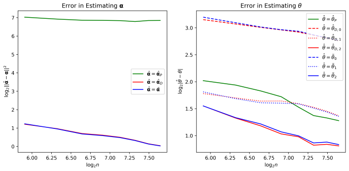
- [Section 4.1, Figure 1] The theoretical rate functions f_α, g_α, h_α and f_θ, g_θ, h_θ are plotted with calibrated constants, but the text does not explicitly state which theorem or corollary each dashed curve corresponds to; adding this mapping would improve reproducibility.
- [Section 5.3.1] In the proof of Theorem 2(b), the chi-squared calculations are stated to follow from Lemma A.1 of Fan, Rigollet, and Wang (2015); since this lemma is central to the lower bound, stating it explicitly in Section 5.9 would make the proof more self-contained.
Circularity Check
No circularity: the minimax lower and upper bounds are derived from explicit data-generating constructions and concentration inequalities, with self-citations only to peripheral technical lemmas.
full rationale
The derivation chain is self-contained. The upper bounds (Theorems 1 and 4) follow from KKT identities, the cone/restricted-eigenvalue lemmas (Lemmas 3–4), and standard concentration inequalities (Lemmas 1–2); the constants are selected from the parameter-class bounds, not from the target error rates. The lower bounds (Theorems 2 and 5) are obtained from explicit two-point and two-fuzzy-hypothesis Gaussian constructions with computed KL/χ² divergences, independently of the estimator's form; Proposition 1 is a by-product of these constructions. The only self-citation that enters the proof, Fan, Rigollet, and Wang (2015), supplies a generic algebraic bound on χ² divergence for Gaussian mixtures (their Lemma A.1); it does not contain the target functional's rate and is parameter-free with stated assumptions, so it is genuine external support rather than a load-bearing self-citation. The robust-input results cited from Ke et al. and the de-biasing references (Zhang–Zhang, Javanmard–Montanari) are similarly auxiliary. No fitted parameter is renamed as a prediction, and no quantity is defined in terms of the target. The apparent failure of the displayed approximate-sparsity rates to reduce to Corollary 1 when q = 0 is an internal consistency and correctness concern in Section 3.4, not a circularity: it does not make the claimed rates equivalent to the paper's inputs by construction.
Assumptions & free parameters
free parameters (1)
- Simulation tuning parameters (λ, γ) in Section 4.1 =
unknown, chosen to minimize estimation error
assumptions (4)
- domain assumption Sub-gaussianity of x = Σ^{1/2} y + μ with ||y||_{ψ2} = ν as in (2.1).
- domain assumption Eigenvalue bounds c_L ≤ λ_min(Σ) ≤ δ_Σ ≤ c_U for fixed constants c_L, c_U > 0.
- domain assumption Sparsity of α = Σ^{-1} μ: exact (H(s,τ)) or approximate (H_q(R,τ)).
- standard math Standard concentration inequalities (Hoeffding, Bernstein, matrix deviation) from Vershynin (2018) and related references.
Cite this review
Pith. "Pith review of Optimal estimation of functionals of high-dimensional mean and covariance matrix." pith.science (2026). https://pith.science/paper/SQGHEIYA
@misc{pith2026190807460,
  author       = {Pith},
  title        = {Pith review of: Optimal estimation of functionals of high-dimensional mean and covariance matrix},
  year         = {2026},
  howpublished = {\url{https://pith.science/paper/SQGHEIYA}},
  note         = {Machine review of arXiv:1908.07460}
}
abstract
Motivated by portfolio allocation and linear discriminant analysis, we consider estimating a functional $\mathbf{\mu}^T \mathbf{\Sigma}^{-1} \mathbf{\mu}$ involving both the mean vector $\mathbf{\mu}$ and covariance matrix $\mathbf{\Sigma}$. We study the minimax estimation of the functional in the high-dimensional setting where $\mathbf{\Sigma}^{-1} \mathbf{\mu}$ is sparse. Akin to past works on functional estimation, we show that the optimal rate for estimating the functional undergoes a phase transition between regular parametric rate and some form of high-dimensional estimation rate. We further show that the optimal rate is attained by a carefully designed plug-in estimator based on de-biasing, while a family of naive plug-in estimators are proved to fall short. We further generalize the estimation problem and techniques that allow robust inputs of mean and covariance matrix estimators. Extensive numerical experiments lend further supports to our theoretical results.
Figures

Figures from the paper (3 more)


Reference graph
Works this paper leans on
-
[1]
Anderson, T. (2003). An Introduction to Multivariate Statistical Analysis, 3rd Edition . Wiley- Interscience
2003
-
[2]
Ao, M., Li, Y., and Zheng, X. (2017). Solving the Markowitz Optimization Problem for Large Portfolios. Manuscript
2017
-
[3]
Bai, Z., Liu, H., and Wong, W. (2009). Enhancement of the applicability of Markowitz’s portfolio optimization by utilizing random matrix theory. Mathematical Finance, 19(4), 639–667
2009
-
[4]
Bai, Z. and Sarandasa, H. (1996). Effect of High Dimension: By an Example of a Two Sample Problem. Statistica Sinica, 6, 311–329
work page 1996
-
[5]
Bai, Z., Silverstein, J., and Yin, Y. (1988). A note on the largest eigenvalue of a large dimensional sample covariance matrix. Journal of Multivariate Analysis , 26, 166–168. 83
work page 1988
-
[6]
Bai, Z. and Yin, Y. (1993). Limit of the smallest eigenvalue of large dimensional sample covariance matrix. Annals of Probability, 21, 1275–1294
work page 1993
-
[7]
Bickel, P. and Levina, E. (2004). Some theory for Fisher’s linear discriminant function, ‘naive Bayes’, and some alternatives when there are many more variables than observations. Bernoulli, 10, 989–1010
work page 2004
-
[8]
Bickel, P. and Ritov, Y. (1988). Estimating integrated squared density derivatives: Sharp best order of convergence estimates. Sankhy¯ a Ser. A, 50, 381–393
work page 1988
Show all 83 references
-
[9]
Bickel, P., Ritov, Y., and Tsybakov, A. (2009). Simultaneous analysis of Lasso and Dantzig selector. Annals of Statistics , 37(4), 1705–1732. Birg´ e, L. and Massart, P. (2001). Gaussian model selection.Journal of the European Mathematical Society, 3(3), 203–268
2009
-
[10]
Boucheron, S., Lugosi, G., and Massart, P. (2013). Concentration inequalities: A nonasymptotic theory of independence. Oxford University Press
2013
-
[11]
Brodie, J., Daubechies, I., De Mol, C., Giannone, D., and Loris, I. (2009). Sparse and stable Markowitz portfolios. Proceedings of the National Academy of Sciences , 106(30), 12267–12272. B¨ uhlmann, P. and van de Geer, S. (2011). Statistics for high-dimensional data: methods,...
2009
-
[12]
Butucea, C. (2007). Goodness-of-fit testing and quadratic functional estimation from indirect ob- servations. Annals of Statistics , 35, 1907–1930
2007
-
[13]
and Comte, F
Butucea, C. and Comte, F. (2009). Adaptive estimation of linear functionals in the convolution model and applications. Bernoulli, 15, 69–98
2009
-
[14]
and Guo, Z
Cai, T. and Guo, Z. (2017). Confidence intervals for high-dimensional linear regression: Minimax rates and adaptivity. Annals of Statistics , 45(2), 615–646
2017
-
[15]
Cai, T., Liu, W., and Xia, Y. (2014). Two-sample test of high dimensional means under dependence. J.R.Statist. Soc. B , 76, 349–372
2014
-
[16]
and Low, M
Cai, T. and Low, M. (2004). Minimax estimation of linear functionals over nonconvex parameter spaces. Annals of Statistics , 32(2), 552–576. 84
2004
-
[17]
Cai, T., Ren, Z., and Zhou, H. (2016). Estimating structured high-dimensional covariance and precision matrices: Optimal rates and adaptive estimation. 10, 1–59
2016
-
[18]
and Yuan, M
Cai, T. and Yuan, M. (2012). Adaptive covariance matrix estimation through block thresholding. Annals of Statistics , 40, 2014–2042
2012
-
[19]
Cai, T., Zhang, C., and Zhou, H. (2010). Optimal rates of convergence for covariance matrix estimation. Annals of Statistics , 38(4), 2118–2144
2010
-
[20]
and Zhang, L
Cai, T. and Zhang, L. (2018). High-dimensional Linear Discriminant Analysis: Optimality, Adap- tive Algorithm, and Missing Data. Manuscript
2018
-
[21]
and Zhou, H
Cai, T. and Zhou, H. (2012). Optimal rates of convergence for sparse covariance matrix estimation. Annals of Statistics , 40(5), 2389–2420. Cand` es, E. and Tao, T. (2007). The Dantzig selector: Statistical estimation whenp is much larger than n. Annals of Statistics , 35(6), ...
2012
-
[22]
and Qin, Y
Chen, S. and Qin, Y. (2010). A Two-sample Test for High-dimensional Data with Application to Gene-Set Testing. Annals of Statistics , 38, 808–835
2010
-
[23]
Chen, X., Xu, M., and Wu, W. (2016). Regularized estimation of linear functionals of precision matrices for high-dimensional time series. IEEE Transactions on Signal Processing , 64(24), 6459–6470
2016
-
[24]
Collier, O., Comminges, L., and Tsybakov, A. (2017). Minimax estimation of linear and quadratic functionals on sparsity classes. Annals of Statistics , 45(3), 923–958
2017
-
[25]
and Thomas, J
Cover, T. and Thomas, J. (2012). Elements of information theory . John Wiley & Sons
2012
-
[26]
DeMiguel, V., Garlappi, L., Nogales, J., Uppal, R. (2009). A generalized approach to portfolio optimization: Improving performance by constraining portfolio norms. Management Science , 55(5), 798–812
2009
-
[27]
Devroye, L., Lerasle, M., Lugosi, G., and Oliveira, R. (2016). Sub-Gaussian mean estimators. Annals of Statistics , 44(6), 2695–2725
2016
-
[28]
and Nussbaum, M
Donoho, D. and Nussbaum, M. (1990). Minimax quadratic estimation of a quadratic functional. J. Complexity, 6, 290–323. 85
1990
-
[29]
and Low, M
Efromovich, S. and Low, M. (1996). On optimal adaptive estimation of a quadratic functional. Annals of Statistics , 24, 1106–1125
1996
-
[30]
Fan, J. (1991). On the estimation of quadratic functionals. Annals of Statistics , 19(3), 1273–1294
1991
-
[31]
and Fan, Y
Fan, J. and Fan, Y. (2008). High dimensional classification using features annealed independence rules. Annals of Statistics , 36, 2605–2637
2008
-
[32]
Fan, J., Fan, Y., and Lv, J. (2008). High dimensional covariance matrix estimation using a factor model. Journal of Econometrics , 147, 186–197
2008
-
[33]
Fan, J., Han, F., and Liu, H. (2014). Challenges of big data analysis. National science review, 1(2), 293–314
2014
-
[34]
and Li, R
Fan, J. and Li, R. (2001). Variable selection via nonconcave penalized likelihood and its oracle properties. Journal of the American Statistical Association , 96, 1348–1360
2001
-
[35]
Fan, J., Liao, Y., and Liu, H. (2016). An overview of the estimation of large covariance and precision matrices. Econometrics Journal, 19, 1–32
2016
-
[36]
Fan, J., Liao, Y., and Mincheva, M. (2013). High-dimensional covariance matrix estimation in approximate factor models. Annals of Statistics , 39, 3320–3356
2013
-
[37]
Fan, J., Liao, Y., and Mincheva, M. (2013). Large covariance estimation by thresholding principal orthogonal complements. J. R. Statisti. Soc. B , 75, 603–680
2013
-
[38]
and Lv, J
Fan, J. and Lv, J. (2008). Sure independence screening for ultrahigh dimensional feature space. Journal of the Royal Statistical Society: Series B (Statistical Methodology) , 70(5), 849–911
2008
-
[39]
and Lv, J
Fan, J. and Lv, J. (2018). Sure independence screening.Wiley StatsRef: Statistics Reference Online, 1–8
2018
-
[40]
Fan, J., Rigollet, P., and Wang, W. (2015). Estimation of functionals of sparse covariance matrices. Annals of Statistics , 43(6), 2706–2737
2015
-
[41]
Fan, J., Wang, K., Zhong, Y., and Zhu, Z. (2018). Robust high dimensional factor models with applications to statistical machine learning. Statistical Science, invited
2018
-
[42]
Fan, J., Zhang, J., and Yu, K. (2012). Vast portfolio selection with gross exposure constraints. Journal of the American Statistical Association , 107(498), 592–606
2012
-
[43]
Fan, J., Wang, W., and Zhu, Z.W. (2021+). A shrinkage principle for heavy-tailed data: High- dimensional robust low-rank matrix recovery. Annals of Statistics , to appear
2021
-
[44]
and Bengtsson, T
Furrer, R. and Bengtsson, T. (2007). . Estimation of high-dimensional prior and posterior covariance matrices in Kalman filter variants. Journal of Multivariate Analysis , 98(2), 227–255
2007
-
[45]
Guo, Z., Wang, W., Cai, T., and Li, H. (2018). Optimal Estimation of Genetic Relatedness in High-Dimensional Linear Models. Journal of the American Statistical Association , 0, 1–12
2018
-
[46]
and Khas’minskii, R
Ibragimov, I. and Khas’minskii, R. (1984). Nonparametric estimation of the value of a linear func- tional in Gaussian white noise. Theory Probab. Appl., 29, 18–32. 86
1984
-
[47]
and Montanari, A
Javanmard, A. and Montanari, A. (2014). Confidence intervals and hypothesis testing for high dimensional regression. Journal of Machine Learning Research, , 15(1), 2869–2909
2014
-
[48]
and Montanari, A
Javanmard, A. and Montanari, A. (2014). Hypothesis Testing in High-Dimensional Regression under the Gaussian Random Design Model: Asymptotic Theory.IEEE Trans. on Inform. Theory, 60(10), 6522–6554
2014
-
[49]
and Montanari, A
Javanmard, A. and Montanari, A. (2018). Debiasing the lasso: Optimal sample size for Gaussian designs. Annals of Statistics , 46(6), 2593–2622
2018
-
[50]
Johnstone, I. (2001). On the distribution of the largest eigenvalue in principal components analysis. Annals of Statistics , 29, 295–327
2001
-
[51]
and Lu, Y
Johnstone, I. and Lu, Y. (2009). On consistency and sparsity for principal components analysis in high dimensions. Journal of the American Statistical Association , 104(486), 682–693
2009
-
[52]
and Titterington, M
Johnstone, I. and Titterington, M. (2009). Statistical challenges of high-dimensional data. Phil. Trans. R. Soc. A, 364, 4237–4253
2009
-
[53]
and Zhou, G
Kan, R. and Zhou, G. (2007). Optimal portfolio choice with parameter uncertainty. Journal of Financial and Quantitative Analysis , 42(3), 621–656
2007
-
[54]
Karoui, N. (2008). Operator norm consistent estimation of large-dimensional sparse covariance matrices. Annals of Statistics , 36(6), 2717–2756
2008
-
[55]
Karoui, N. (2010). High-dimensionality effects in the Markowitz problem and other quadratic pro- grams with linear constraints: Risk underestimation. Annals of Statistics , 38(6), 3487–3566
2010
-
[56]
Ke, Y., Minsker, S., Ren, Z., Sun, Q., and Zhou, W. (2019). User-Friendly Covariance Estimation for Heavy-Tailed Distributions. arXiv:1811.01520. Klemel¨ a, J. and Tsybakov, A. (2001). Sharp adaptive estimation of linear functionals. Annals of Statistics, 29, 1567–1600
2019 arXiv
-
[57]
Koltchinskii, V. (2019). Asymptotically efficient estimation of smooth functionals of covariance operators. arXiv: 1710.09072
2019 arXiv
-
[58]
Koltchinskii, V. (2020). Estimation of smooth functionals in high-dimensional models: bootstrap chains and Gaussian approximation. arXiv: 2011.03789
2020 arXiv
-
[59]
and Zhilova, M
Koltchinskii, V. and Zhilova, M. (2019). Estimation of smooth functionals in normal models: bias reduction and asymptotic efficiency. arXiv: 1912.08877
2019 arXiv
-
[60]
and Fan, J
Lam, C. and Fan, J. (2009). Sparsistency and rates of convergence in large covariance matrix estimation. Annals of Statistics , 37, 4254–4278
2009
-
[61]
and Massart, P
Laurent, B. and Massart, P. (2000). Adaptive estimation of a quadratic functional by model selec- tion. Annals of Statistics , 28, 1302–1338
2000
-
[62]
and Wainwright, M
Loh, P. and Wainwright, M. (2017). Support recovery without incoherence: A case for nonconvex regularization. Annals of Statistics , 45(6), 2455–2482. 87
2017
-
[63]
Markowitz, H. (1952). Portfolio selection. Journal of Finance , 7, 77–91
1952
-
[64]
Mai, Q. (2013). A review of discriminant analysis in high dimensions. Computational Statistics, 5, 190–197
2013
-
[65]
A direct approach to sparse discriminant analysis in ultra- high dimensions
Mai, Q., Zou, H., and Yuan, M.(2012). A direct approach to sparse discriminant analysis in ultra- high dimensions. Biometrika, 99, 29–42
2012
-
[66]
Negahban, S., Ravikumar, P., Wainwright, M., and Yu, B. (2012). A unified framework for high- dimensional analysis of M-estimators with decomposable regularizers. Statistical Science, 27(4), 538–557
2012
-
[67]
Nemirovskii, A. (2000). Topics in nonparametric statistics. Lectures on Probability Theory and Statistics (Saint-Flour, 1998). Lecture Notes in Math . 1738, 85–277. Springer, Berlin
2000
-
[68]
Paul, D. (2007). Asymptotics of sample eigenstructure for a large dimensional spiked covariance model. Statistica Sinica, 17, 1617–1642
2007
-
[69]
Raskutti, G., Wainwright, M., and Yu, B. (2010). Restricted eigenvalue properties for correlated Gaussian designs. Journal of Machine Learning Research , 11, 2241–2259
2010
-
[70]
and Wang, S
Shao, J., Wang, Y., Deng, X. and Wang, S. (2011). Sparse linear discriminant analysis with high dimensional data. Annals of Statistics , 39, 1241–1265
2011
-
[71]
Srivastava, M. (2009). A test for the mean vector with fewer observations than the dimension under non-normality. Journal of Multivariate Analysis , 100, 518–532
2009
-
[72]
and Du, M
Srivastava, M. and Du, M. (2008). A Test for the Mean Vector with Fewer Observations than the Dimension. Journal of Multivariate Analysis , 99, 386–402
2008
-
[73]
Sun, Q., Zhou, W., and Fan, J. (2018). Adaptive huber regression. Journal of the American Sta- tistical Association, 1–35
2018
-
[74]
Tibshirani, R. (1996). Regression shrinkage and selection via the lasso. Journal of the Royal Sta- tistical Society. Series B , 58(1), 267–288
1996
-
[75]
Tsybakov, A. (2009). Introduction to Nonparametric Estimation. Springer, New York. Van de Geer, S., B¨ uhlmann, P., Ritov, Y., and Dezeure, R. (2014). On asymptotically optimal confidence regions and tests for high-dimensional models. Annals of Statistics, 42(3), 1166–1202. Van...
2009
-
[76]
Vershynin, R. (2010). Introduction to the non-asymptotic analysis of random matrices. arXiv:1011.3027
2010 arXiv
-
[77]
Vershynin, R. (2018). High-dimensional probability: An introduction with applications in data sci- ence. Cambridge University Press. Von Rosen, D. (1988). Moments for the inverted Wishart distribution. Scandinavian Journal of Statistics, 15, 97–109. 88
2018
-
[78]
Wainwright, M. (2019). High-dimensional statistics: a non-asymptotic viewpoint . Cambridge Uni- versity Press
2019
-
[79]
Wang, L., Peng, B., and Li, R. (2015). A High-Dimensional Nonparametric Multivariate Test for Mean Vector. Journal of the American Statistical Association , 110, 1658–1669
2015
-
[80]
and Fan, J
Wang, W. and Fan, J. (2017). Asymptotics of empirical eigen-structure for high dimensional spiked covariance. Annals of Statistics , 45, 1342-1374
2017
-
[81]
Zhang, C. (2010). Nearly unbiased variable selection under minimax concave penalty. The Annals of Statistics, 38, 894–942
2010
-
[82]
and Zhang, S
Zhang, C. and Zhang, S. (2014). Confidence intervals for low dimensional parameters in high dimen- sional linear models. Journal of the Royal Statistical Society: Series B (Statistical Methodology) , 76(1), 217–242
2014
-
[83]
Zhong, P., Chen, S., and Xu, M. (2013). Tests alternative to higher criticism for high-dimensional means under sparsity and column-wise dependence. Annals of Statistics , 6, 2820–2851. 89
2013
Reviewed August 14, 2026 · model on record in the stance chip above.
Discussion (0). Continue with ORCID to comment.