REVIEW 2 major objections 5 minor 33 references
Measurements Number Scaling in the Quantum Approximate Optimization Algorithm for MaxCut: A Statistical Analysis
T0 review · 2 major / 5 minor · reviewed 2026-07-12 · grok-4.5
Pith's one-line read For large MaxCut graphs of fixed local structure, QAOA needs fewer measurement shots to hit the same relative accuracy as the graph grows.
desk verdict Clean, usable inverse-shot scaling for relative-error QAOA MaxCut under extensivity; the math holds and the result is new relative to the concentration literature. read the letter →
The pith
A machine-rendered reading of the paper's core claim, the machinery that carries it, and where it could break.
The reading
What carries the argument
Relative concentration of the MaxCut cost: both expectation and variance scale linearly with m, so the relative standard deviation shrinks as 1/√m; Janson’s inequality then yields an inverse shot bound, and the same scaling plus PL/Lipschitz assumptions carries the argument through SGD.
What would settle it
On a sequence of bounded-degree graphs that keep the same local structure, measure the minimal shots needed to keep relative cost error below a fixed δ with fixed confidence: if that shot count does not fall roughly as 1/m, the central scaling claim is false.
Extended reading notes
Core claim
Under an extensive-cost lower bound and linear scaling of the Polyak-Łojasiewicz and Lipschitz constants, a sufficient shot budget per QAOA cost evaluation that guarantees fixed relative estimation error (or fixed relative SGD suboptimality) decreases as 1/m with the number of edges m, while the iteration count remains Θ(1).
Load-bearing premise
The expected QAOA cost must stay at least a fixed positive fraction of the number of edges throughout the optimization; if the cost stops being extensive, the inverse-shot claim fails.
Editorial extensions
If this is right
- For Benjamini–Schramm convergent families (regular, sparse Erdős–Rényi, cycles) the total shot budget for fixed relative performance improves with size.
- Angle-transfer methods that already avoid outer-loop optimization can also run with a shrinking measurement budget.
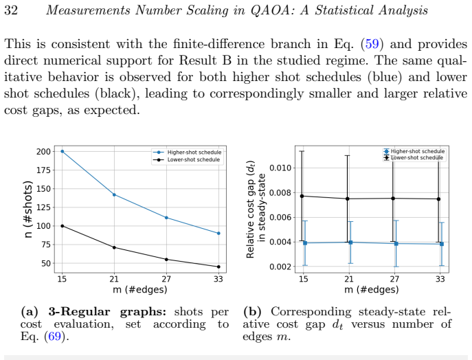
- Finite-difference gradient estimators inherit the 1/m shot scaling; gate-wise parameter-shift estimators keep a size-independent shot count.
- Practitioners can calibrate shots on small graphs and extrapolate by the inverse-size rule for larger instances of the same family.
Reading between the lines
- The same relative-concentration argument may apply to other local-cost combinatorial problems (e.g., Max-k-SAT or Ising models with bounded degree) once an extensive lower bound is verified.
- If absolute rather than relative accuracy is required, as in many VQE energy targets, the 1/m advantage disappears.
- Hardware-aware implementations that already use shallow fixed-angle QAOA could further cut classical post-processing by deliberately lowering the shot schedule with instance size.
Signed reviews
Editorial analysis
A structured set of objections, weighed in public.
Referee Report
Summary. The manuscript analyzes the measurement (shot) complexity of QAOA for MaxCut. Using Janson’s inequality on dependent edge terms and standard L-smooth + Polyak–Łojasiewicz SGD theory, it derives sufficient shot budgets to (a) estimate the cost to relative error δ with confidence 1−ε and (b) keep the SGD relative suboptimality below a target ξ*. Under an extensive-cost lower bound |⟨Cp⟩|≥κm and linear scaling of the PL and Lipschitz constants (Assumptions 1–3), the sufficient shots per cost evaluation scale as 1/m for finite-difference gradients (and as Θ(1) for parameter-shift), while the number of SGD iterations is Θ(1). The authors characterize the relevant graph classes via Benjamini–Schramm local limits, give practitioner calibration rules, and support the scalings with noiseless finite-shot simulations on regular, sparse Erdős–Rényi, and random connected graphs.
Significance. If the extensivity and linear PL/Lipschitz hypotheses hold for the intended families, the result is a genuine and useful contribution: it shows that a fixed relative performance target can become cheaper in shots as MaxCut instances grow, complementing known parameter-transfer / tree-QAOA concentration results. The finite-difference versus parameter-shift variance prefactors are treated carefully, the concentration argument via Janson is correctly applied to QAOA causal cones, and the paper supplies explicit sufficient conditions, practitioner heuristics, and public code. The claims are properly conditional rather than universal, which is appropriate. Strengths include transparent derivations, local-positivity lemmas supporting extensivity, and numerical checks that track the predicted 1/m trend on small but structured instances.
major comments (2)
- Assumption 1 (and Appendix A, Reasoning I) is load-bearing for the 1/m claim. Reasoning I lower-bounds |⟨Cp⟩| by m/2 using the (0,0) initialization together with monotonicity of the expected cost along the SGD trajectory. Noisy SGD need not be monotone pathwise. Either restrict the trajectory claim to expected progress / noise-free descent, or replace it by a weaker, rigorously controlled condition (e.g., that the optimizer remains in a region where |F|≥κm). Reasoning II (ensemble average under Benjamini–Schramm) and the local-positivity lemmas already give a cleaner route; elevating that route would remove the gap.
- Assumptions 2–3 and Appendix C.2: the scalings µ=Θ(m) and L=Θ(m) rest on strong convexity of the limiting per-edge objective on a local region U. That landscape hypothesis is not checked numerically (e.g., Hessian spectra or empirical PL constants on the calibration graphs). Because Results B–C and the claim T=Θ(1) depend on µ/L=Θ(1), a short numerical check or a more prominent caveat that the iteration/shot conclusions are conditional on this local strong-convexity property would make the load-bearing hypothesis transparent.
minor comments (5)
- Notation for the sample mean of the cost is inconsistent in places (ˆCp vs ⟨ˆCp⟩, e.g. Lemma 3 / Appendix B). Pick one convention and use it throughout.
- Fig. 4 reports minimal shot counts from a single graph instance per size; adding error bars or medians over the 10 instances already used elsewhere would better match the multi-instance protocol of Figs. 3 and 6–8.
- In Sec. 4.3 the relative gap dt is evaluated from exact state-vector costs while only the gradient is shot-noisy. This is fine for testing the theory, but the practitioner heuristics (Sec. 3.5) should note that full shot noise on both cost and gradient may require a modestly larger budget.
- Typographical: “Polyak- Lojasiewicz” should be “Polyak–Łojasiewicz” (or “Polyak-Lojasiewicz”) consistently; a few missing spaces after commas appear in the abstract and Sec. 1.
- The open Conjecture 10 is interesting but not needed for the main theorems; a one-sentence pointer that the proved lemmas already cover the tree-like and path-repeatable cases used in the scaling claims would help readers.
Circularity Check
No significant circularity: shot-scaling bounds follow from external concentration inequalities plus scoped extensivity/PL assumptions justified by independent local-limit arguments; only minor non-load-bearing self-reference to prior tree-QAOA work.
full rationale
The central claims (Result A: np = Ω(1/m) for fixed relative error δ under |Fp| ≥ κ m; Result B: same for finite-difference SGD under μ = Θ(m); Result C: T = Θ(1) under L = Θ(m)) are derived from Janson’s inequality (Eq. 2 / Lemma 3), the Farhi et al. variance bound Var(C) ≤ 2 cvp m (Eq. 34), and standard L-smooth + PL SGD analysis (Lemma 5, Thm. 4/6). Assumptions 1–3 are explicitly stated and supported by external Benjamini–Schramm convergence plus original local-positivity lemmas (App. A Lemmas 7–9) and Hessian-convergence arguments (App. C.2); none of these reduce the target scaling to a fitted constant or to a definition. Numerical experiments independently check the predicted scalings rather than fitting and re-predicting. The only self-reference is a non-load-bearing complement to prior tree-QAOA parameter-transfer results (including one co-authored paper), which is not used to force the shot bounds. The derivation chain is therefore self-contained against its stated external inputs and assumptions.
Assumptions & free parameters
assumptions (6)
- domain assumption Assumption 1: |Fp(θ;G)| ≥ κ m for some κ > 0 independent of m (extensive cost).
- domain assumption Assumption 2: the PL constant satisfies μ = Θ(m).
- domain assumption Assumption 3: the gradient Lipschitz constant satisfies L = Θ(m).
- standard math Janson’s inequality for dependent summands with maximum dependency degree Λ ≤ 2 c_vp.
- domain assumption Local invexity / PL inequality holds in the region reached by the SGD trajectory.
- domain assumption Variance bound Var(C) ≤ 2 c_vp m of Farhi et al. (2014).
Cite this review
Pith. "Pith review of Measurements Number Scaling in the Quantum Approximate Optimization Algorithm for MaxCut: A Statistical Analysis." pith.science (2026). https://pith.science/paper/SS6VWHLM
@misc{pith2026260703340,
  author       = {Pith},
  title        = {Pith review of: Measurements Number Scaling in the Quantum Approximate Optimization Algorithm for MaxCut: A Statistical Analysis},
  year         = {2026},
  howpublished = {\url{https://pith.science/paper/SS6VWHLM}},
  note         = {Machine review of arXiv:2607.03340}
}
abstract
We provide a statistical analysis of the measurement (shot) requirements of the quantum approximate optimization algorithm (QAOA) for the MaxCut problem. We derive sufficient conditions on the number of shots per cost operator evaluation to: (a) estimate the expected cost to within a relative error $\delta$ and a confidence $1-\epsilon$, and (b) ensure SGD-based parameter optimization converges to a target relative suboptimality level with high probability. In addition, we provide an explicit bound on the number of SGD iterations required to reach the target accuracy. Our analysis reveals an unexpected scaling phenomenon: for specific graph classes, which we formally characterize, the total shot budget needed to achieve a fixed relative-performance metric decreases as the instance size grows. This result complements earlier cost function concentration arguments regarding parameter optimization redundancy, thereby highlighting the potential for high-performance, low-overhead QAOA implementations for large-scale MaxCut instances. To assist practitioners, we translate our analytical findings into practical rules of thumb for shot-budget allocation and validate these results with numerical simulations, offering new insights into the interplay between graph size, structural complexity, and resource requirements in QAOA.
Figures


Figures from the paper (5 more)



Reference graph
Works this paper leans on
-
[1]
Farhi, E., Goldstone, J., Gutmann, S.: A Quantum Approximate Opti- mization Algorithm. arXiv. https://doi.org/10.48550/arXiv.1411.4028. http://arxiv.org/abs/1411.4028
-
[2]
Kashapogu, R., Hasib, S., Rasool, A.: Exploring the Versatility of QAOA: A Comprehensive Review. (2024). https://doi.org/10.1109/ ICCCNT61001.2024.10725610
arXiv 2024
-
[3]
Nature Reviews Physics3(9), 625–644 (2021)
Cerezo, M., Arrasmith, A., Babbush, R., Benjamin, S.C., Endo, S., Fujii, K., McClean, J.R., Mitarai, K., Yuan, X., Cincio, L.,et al.: Variational quantum algorithms. Nature Reviews Physics3(9), 625–644 (2021). https: //doi.org/10.1038/s42254-021-00348-9
-
[4]
https://arxiv.org/abs/1812.04170
Brandao, F.G.S.L., Broughton, M., Farhi, E., Gutmann, S., Neven, H.: For Fixed Control Parameters the Quantum Approximate Optimization Algorithm’s Objective Function Value Concentrates for Typical Instances (2018). https://arxiv.org/abs/1812.04170
arXiv 2018
-
[5]
Physical Review X10(2), 021067 (2020)
Zhou, L., Wang, S.-T., Choi, S., Pichler, H., Lukin, M.D.: Quan- tum approximate optimization algorithm: Performance, mechanism, and implementation on near-term devices. Physical Review X10(2), 021067 (2020). https://doi.org/10.1103/PhysRevX.10.021067
-
[6]
Wauters, M.M., Mbeng, G.B., Santoro, G.E.: Polynomial scaling of the quantum approximate optimization algorithm for ground-state prepa- ration of the fully connectedp-spin ferromagnet in a transverse field. Phys. Rev. A102, 062404 (2020). https://doi.org/10.1103/PhysRevA. 102.062404
doi:10.1103/physreva 2020
-
[7]
Wang, Z., Hadfield, S., Jiang, Z., Rieffel, E.G.: Quantum approximate optimization algorithm for MaxCut: A fermionic view97(2), 022304. Measurements Number Scaling in QAOA: A Statistical Analysis51 https://doi.org/10.1103/PhysRevA.97.022304. Accessed 2024-11-16
-
[8]
In: Proceedings of the 21st ACM International Conference on Computing Frontiers, pp
Rajakumar, J., Golden, J., B¨ artschi, A., Eidenbenz, S.: Trainability bar- riers in low-depth qaoa landscapes. In: Proceedings of the 21st ACM International Conference on Computing Frontiers, pp. 199–206 (2024). https://doi.org/10.1145/3649153.3649204
Show all 33 references
-
[9]
Nature Reviews Physics, 1–16 (2025)
Larocca, M., Thanasilp, S., Wang, S., Sharma, K., Biamonte, J., Coles, P.J., Cincio, L., McClean, J.R., Holmes, Z., Cerezo, M.: Barren plateaus in variational quantum computing. Nature Reviews Physics, 1–16 (2025). https://doi.org/10.1038/s42254-025-00813-9
2025 doi
-
[10]
Quantum5, 491 (2021)
Sack, S.H., Serbyn, M.: Quantum annealing initialization of the quantum approximate optimization algorithm. Quantum5, 491 (2021). https:// doi.org/10.22331/q-2021-07-01-491
2021 doi
-
[11]
Quantum Machine Intelligence6(2), 38 (2024)
Amosy, O., Danzig, T., Lev, O., Porat, E., Chechik, G., Makmal, A.: Iteration-free quantum approximate optimization algorithm using neural networks. Quantum Machine Intelligence6(2), 38 (2024). https://doi.org/ 10.1007/s42484-024-00159-y
2024 doi
-
[12]
https: //arxiv.org/abs/1908.08862
Streif, M., Leib, M.: Training the Quantum Approximate Optimization Algorithm without access to a Quantum Processing Unit (2019). https: //arxiv.org/abs/1908.08862
2019 arXiv
-
[13]
Wurtz, J., Lykov, D.: Fixed-angle conjectures for the quantum approx- imate optimization algorithm on regular maxcut graphs. Phys. Rev. A 104, 052419 (2021). https://doi.org/10.1103/PhysRevA.104.052419
2021 doi
-
[14]
Quantum9, 1892 (2025)
Wybo, E., Leib, M.: Missing puzzle pieces in the performance landscape of the quantum approximate optimization algorithm. Quantum9, 1892 (2025). https://doi.org/10.22331/q-2025-10-22-1892
2025 doi
-
[15]
https: //arxiv.org/abs/2503.12789
Farhi, E., Gutmann, S., Ranard, D., Villalonga, B.: Lower bounding the MaxCut of high girth 3-regular graphs using the QAOA (2025). https: //arxiv.org/abs/2503.12789
2025
-
[16]
Random Structures and Algorithms24(2004)
Janson, S.: Large deviations for sums of partly dependent random vari- ables. Random Structures and Algorithms24(2004). https://doi.org/10. 1002/rsa.20008
2004
-
[17]
Physical Review A99(3), 032331 (2019)
Schuld, M., Bergholm, V., Gogolin, C., Izaac, J., Killoran, N.: Evaluat- ing analytic gradients on quantum hardware. Physical Review A99(3), 032331 (2019). https://doi.org/10.1103/PhysRevA.99.032331
2019 doi
-
[18]
https://arxiv.org/abs/1811.04968
Bergholm, V., Izaac, J., Schuld, M., Gogolin, C., Ahmed, S., Ajith, V., Alam, M.S., Alonso-Linaje, G., AkashNarayanan, B., Asadi, A., Arrazola, 52Measurements Number Scaling in QAOA: A Statistical Analysis J.M., Azad, U., Banning, S., Blank, C., Bromley, T.R., Cordier, B.A., C...
2022 arXiv
-
[19]
https://github.com/PennyLaneAI/pennylane
Accessed: 2023-03-23. https://github.com/PennyLaneAI/pennylane
2023
-
[20]
Quantum6, 677 (2022)
Wierichs, D., Izaac, J., Wang, C., Lin, C.Y.-Y.: General parameter-shift rules for quantum gradients. Quantum6, 677 (2022). https://doi.org/10. 22331/q-2022-03-30-677
2022
-
[21]
https://www-m5.ma.tum.de/foswiki/pub/M5/Allgemeines/ MA4801 2018S/ML notes main.pdf
Wolf, M.M.: Mathematical Foundations of Supervised Learning (2018). https://www-m5.ma.tum.de/foswiki/pub/M5/Allgemeines/ MA4801 2018S/ML notes main.pdf
2018
-
[22]
Electronic Journal of Probability6(none), 1–13 (2001)
Benjamini, I., Schramm, O.: Recurrence of Distributional Limits of Finite Planar Graphs. Electronic Journal of Probability6(none), 1–13 (2001). https://doi.org/10.1214/EJP.v6-96
2001 doi
-
[23]
MIT OpenCourseWare, 18.S096: Topics in Mathematics of Data Science (Fall 2015), Lec- ture Notes
Rahman, M.: Session 17: Local Convergence of Graphs and Enu- meration of Spanning Trees. MIT OpenCourseWare, 18.S096: Topics in Mathematics of Data Science (Fall 2015), Lec- ture Notes. Accessed 2026-02-15 (2015). https://ocw.mit.edu/ courses/18-s096-topics-in-mathematics-of-d...
2015
-
[24]
Lecture notes / book draft
van der Hofstad, R.: Random Graphs and Complex Networks, Volume I. Lecture notes / book draft. Accessed 2026-02-18 (2017). https://rhofstad. win.tue.nl/NotesRGCN.pdf
2026
-
[25]
https: //doi.org/10.22331/q-2024-01-18-1231
Sureshbabu, S.H., Herman, D., Shaydulin, R., Basso, J., Chakrabarti, S., Sun, Y., Pistoia, M.: Parameter setting in quantum approximate opti- mization of weighted problems8, 1231 2305.15201 [quant-ph]. https: //doi.org/10.22331/q-2024-01-18-1231. Accessed 2024-11-16
-
[26]
https://arxiv.org/abs/2005.08747 Measurements Number Scaling in QAOA: A Statistical Analysis53
Farhi, E., Gamarnik, D., Gutmann, S.: The Quantum Approximate Opti- mization Algorithm Needs to See the Whole Graph: Worst Case Examples (2020). https://arxiv.org/abs/2005.08747 Measurements Number Scaling in QAOA: A Statistical Analysis53
2020 arXiv
-
[27]
Physics Reports986, 1–128 (2022)
Tilly, J., Chen, H., Cao, S., Picozzi, D., Setia, K., Li, Y., Grant, E., Woss- nig, L., Rungger, I., Booth, G.H., Tennyson, J.: The variational quantum eigensolver: A review of methods and best practices. Physics Reports986, 1–128 (2022). https://doi.org/10.1016/j.physrep.2022.08.003
2022 doi
-
[28]
Journal of Chemical Theory and Computation20(6), 2390–2403 (2024)
Zhu, L., Liang, S., Yang, C., Li, X.: Optimizing shot assignment in vari- ational quantum eigensolver measurement. Journal of Chemical Theory and Computation20(6), 2390–2403 (2024). https://doi.org/10.1021/acs. jctc.3c01113
2024 doi
-
[29]
PRX Quantum1, 020312 (2020)
Sanders, Y.R., Berry, D.W., Costa, P.C.S., Tessler, L.W., Wiebe, N., Gidney, C., Neven, H., Babbush, R.: Compilation of fault-tolerant quan- tum heuristics for combinatorial optimization. PRX Quantum1, 020312 (2020). https://doi.org/10.1103/PRXQuantum.1.020312
2020 doi
- [30]
-
[31]
https://arxiv.org/abs/1401
Lyons, R.: Factors of IID on Trees (2016). https://arxiv.org/abs/1401. 4197
2016
-
[32]
Accessed: 2023-03-23 (2023)
PennyLane: PennyLane: A Library for Quantum Machine Learning, Quantum Chemistry, and Quantum Optimization. Accessed: 2023-03-23 (2023). https://pennylane.ai/
2023
-
[33]
Applied Optimization, vol
Nesterov, Y.: Introductory Lectures on Convex Optimization: A Basic Course. Applied Optimization, vol. 87. Kluwer Academic Publishers, Boston, MA (2004)
2004
Reviewed July 12, 2026 · model on record in the stance chip above.
Discussion (0). Continue with ORCID to comment.