REVIEW 3 major objections 5 minor 60 references
A diffusion model trained on isolated attached and lifted flame clips can generate synthetic movies of turbulent flames and even stitch together liftoff and reattachment transitions the model never saw.
Reviewed by Pith at T0; open to challenge. T0 means a machine referee read the full paper against a public rubric. the ladder, T0–T4 →
T0 review · deepseek-v4-flash
2026-08-02 05:55 UTC pith:STOBPS2Z
load-bearing objection A solid conditional generation paper whose transition-synthesis headline outruns the evidence; the core diffusion model for attached/detached flames is worth engaging. the 3 major comments →
Generating synthetic evolution of turbulent flames with an experimental data-based spatiotemporal diffusion model
The pith
A machine-rendered reading of the paper's core claim, the machinery that carries it, and where it could break.
Core claim
The central claim is that an x-prediction flow matching model with a spatiotemporal transformer, operating directly on pixel space-time slabs, can conditionally generate whole trajectories (10 or 100 frames) that match the large-scale structure and statistical behavior of real attached and detached swirl flames across four simultaneous measurement channels. As a stronger extrapolation, the paper claims that by defining the transition denoising velocity as a time-varying linear interpolation of the attached and detached denoising velocities (with a weight vector chosen by the user), the model can synthesize spatiotemporally coherent liftoff and reattachment transitions that were held out of t
What carries the argument
The central object is the conditional denoising velocity in an x-prediction flow matching model. For a slab of noise and a class label (attached or detached), a network predicts the clean slab; the predicted clean slab defines a velocity that integrates from noise to data. A spatiotemporal transformer, operating on patches of the space-time slab, supplies the network. For transitions, the machinery is a post-training assumption: the transition velocity is the weighted sum of the attached and detached velocities, with a time-varying weight vector that the user chooses to set the direction (liftoff vs reattachment) and the rate (step vs smooth).
Load-bearing premise
The load-bearing assumption is that a flame going from attached to lifted (or back) behaves like a weighted average of the two steady-state behaviors, with the user's chosen weight schedule setting the pace; if that simple average is wrong, the generated transitions are prescribed interpolations rather than learned dynamics.
What would settle it
For a fixed weight vector (e.g., smooth sigmoid centered at frame 50), generate many transition samples and measure, at each physical frame, an observable known to track real transitions: the asymmetry of the OH-PLIF field (e.g., when left-right intensity imbalance exceeds a threshold) or the strength of the ~400 Hz spectral peak associated with the precessing vortex core. In real transitions, the timing and stochastic variability of these markers reflect turbulent dynamics and are not fully prescribed. If, in the synthetic samples, the marker evolution is essentially a deterministic function
If this is right
- Researchers could generate many statistically consistent synthetic flame movies in either regime on demand, without running new experiments, enabling downstream code or analysis development.
- Rare transition events—liftoff and reattachment—can be manufactured at a chosen timescale, providing a data-augmentation path for data-sparse regimes such as combustion extreme events.
- Conditioning on the regime label makes the generator a controllable exploration tool: one can sample diverse realizations of the same macroscopic state and study cycle-to-cycle variability.
- The trade-off between slab length and small-scale fidelity (10 frames preserve spatial statistics better, 100 frames capture detached dynamics better) gives practitioners a clear knob when choosing model configuration.
- The strategy of training on isolated stable regimes and then blending conditions at inference is, if it holds, a general recipe for synthesizing transitions in other multi-regime flow systems.
Where Pith is reading between the lines
- The same class-blending recipe could be tried on other bistable flow phenomena (e.g., blowoff and relight, separation and reattachment of a boundary layer), treating the weight schedule as an external control rather than a learned physical law; the paper's own caveat suggests the controls are not yet physical.
- The observed high-frequency/small-scale undershoot hints that smaller space-time patches or a spectral loss during training could push fine-scale fidelity closer to measurements without losing the large-scale agreement.
- A testable next step is to learn the weight schedule from real held-out transitions—for example, by fitting it to the observed evolution of the asymmetry marker—and then check whether the generator reproduces the full distribution of real transition durations and precursor events, not just the prescribed sigmoid.
- Because the generator can be sampled many times at a fixed weight, it could be used as a Monte Carlo device to estimate the probability of encountering specific flame structures (e.g., local extinction pockets) at a given stage of liftoff, effectively turning a generative model into a statistical table for extreme events.
Editorial analysis
A structured set of objections, weighed in public.
Referee Report
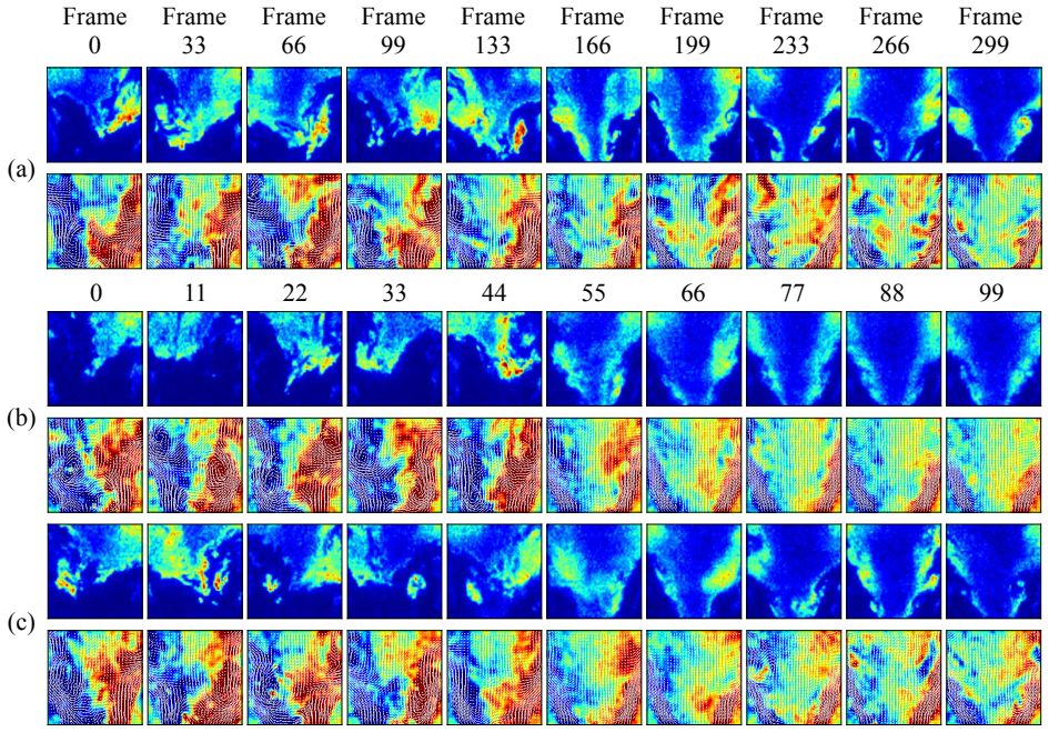
Summary. The paper develops a conditional diffusion model for generating synthetic spatiotemporal trajectories of simultaneous OH-PLIF and three-component PIV measurements in a swirl-stabilized combustor. The model uses an x-prediction flow-matching formulation with a pixel-based spatiotemporal transformer, trained on isolated attached and detached flame slabs (T=10 and T=100 frames). The authors evaluate generation quality via qualitative visualizations, point-probe time traces, POD coefficient statistics, PSD comparisons, and POD spectra, finding good large-scale agreement and modest small-scale deviations. They then propose an extrapolation task: synthesizing flame liftoff/reattachment transitions unseen during training by defining the transition denoising velocity as a time-varying linear combination (Eq. 16) of the attached and detached denoising velocities, with the weight schedule w (Eq. 17) controlling transition direction and timescale. The paper concludes that the approach enables controlled, coherent transition synthesis, with sample-to-sample variability.
Significance. If the central claim holds, the paper offers a useful pathway for data augmentation in data-sparse combustion regimes, especially for extreme events like flame liftoff/reattachment. The work benefits from a clean training/inference formulation (Eqs. 1–6), a detailed architectural description, an explicit T10 vs. T100 comparison, and quantitative POD/PSD-based evaluation of the attached/detached generation task. The authors are admirably candid about limitations, including the observation that the synthetic transitions largely reflect the chosen weight functions. The main unresolved issue is the status of the transition-synthesis claim: it rests entirely on the unvalidated superposition assumption in Eq. 16, and the paper's own discussion (Sec. 4.2.2) acknowledges that the generated transitions are prescribed by the weight schedule rather than learned from data. This is an addressable limitation, so the appropriate recommendation is major revision rather than rejection.
major comments (3)
- [§4.2.1, Eq. (16)] The central novel claim—synthesizing liftoff/reattachment transitions unseen in training—rests on the assumption that the transition denoising velocity is a weighted linear combination of the attached and detached denoising velocities. No derivation from the learned conditional distributions is provided, and no independent empirical validation is given. As the paper itself states in §4.2.2, the synthetic transitions are 'largely a reflection of the weighting functions used to generate them'; this means direction, timing, and rate are prescribed inputs, not emergent dynamics. The only quantitative comparison (Fig. 16) uses a single real transition, with mismatched temporal axes (300 vs. 100 frames) and no error bars or significance testing. The manuscript should either (a) validate Eq. 16 against real held-out transition data—for example, by checking whether Eq. 16 approximates the actual
- [§4.1.3, Figs. 11–12] The statistical comparison for the attached/detached generation task reports mean PSD and POD spectra averaged over 300 samples, but no error bars, confidence intervals, or significance testing are provided. Figures 11 and 12 show small-scale undershoots and high-mode overshoots, yet without uncertainty quantification it is impossible to determine whether these are systematic deficiencies or sampling noise. This is load-bearing for the claim of 'statistical consistency' and should be addressed, for example with bootstrap confidence bands or a quantitative discrepancy measure with confidence intervals.
- [§4.2.2, Fig. 16] Even for the qualitative transition comparison, the real and generated sequences have different lengths (300 frames vs. 100 frames) and are compared on separate time axes. More importantly, only one real transition is used as the baseline (green curves in Fig. 16), and no assessment of run-to-run variability in the real transitions is provided. The synthetic transitions show diverse outcomes for a fixed weight function, but without a distribution of real transitions, the claim that the synthetic trends 'capture the overall evolution trend' is weakly supported. Repeating the comparison over several real transitions and reporting statistics on mean OH evolution would be more convincing.
minor comments (5)
- [Sec. 1] Typo: 'genenrative model' should be 'generative model'.
- [Sec. 4.2.1] In the text following Eq. (16), the notation for the detached velocity is inconsistent: the first occurrence reads 'ˆvs,att = ˆv(zs,τ, 1)' but should presumably be 'ˆvs,det = ˆv(zs,τ, 1)'.
- [Sec. 4.1.2] References to 'Fig. 7(a)' and 'Fig. 7(a)' in the first paragraph should be 'Fig. 8(a)' (and the top-left plot is in Fig. 8(a), not Fig. 7(a)).
- [Fig. 14–16] The frame indices in Figs. 14 and 15 are not aligned between real (0–299) and synthetic (0–99) sequences; while this is acknowledged, the visual comparison would be clearer if the real sequence were cropped to the equivalent transition window or if the axes were labeled with normalized transition progress.
- [Sec. 3.1, Eq. (5)] The derivation of Eq. (5) is correct but could be made more explicit; the rearrangement of Eq. (1) for ε and substitution into v = x − ε is not shown, which may confuse readers.
Circularity Check
Transition synthesis is user-prescribed interpolation (Eqs. 16-17), not an emergent prediction; the attached/detached generator is independently validated.
specific steps
-
self definitional
[Sec. 4.2.1, Eqs. 16-17; Sec. 4.2.2 and Fig. 16]
"the modeled velocity for transition is cast as a weighted linear combination of the modeled velocities for attached and detached flames ... ˆvs,tra(z s,τ)=(1−w)⊙ ˆvs,att(z s,τ)+w⊙ ˆvs,det(z s,τ),(16) ... wi = 1 / (1+exp(−(i−50)/κ)) ... where κ is the squeezing parameter that serves as a synthetic transition timescale. ... the synthetic transitions are largely a reflection of the weighting functions used to generate them"
The transition 'prediction' is not learned from transition data: Eq. 16 defines the transition denoising velocity as a weighted average of the attached and detached velocities, and Eq. 17 sets the weight profile w by user choice. Therefore the direction (liftoff vs reattachment), the midpoint (frame 50), and the rate (κ) of each generated transition are inputs, not outputs inferred from data. The Fig. 16 mean-OH curves consequently track the prescribed w profile, as the paper concedes with 'largely a reflection of the weighting functions.' The comparison to a single real transition uses mismatched 100-frame vs 300-frame axes and no error bars, so it does not independently validate the linear-superposition assumption. Calling this 'synthesizing transitions unseen during training' thus reduc
full rationale
The main generative pipeline is not circular: the attached/detached conditional diffusion model is trained on slabs with transitions explicitly excluded, and its outputs are benchmarked against real data through physical-space visualization, probe time traces, POD spectra, and PSD comparisons. Those checks are external to the model's training objective and provide independent support for the attached/detached generation claims. The only materially circular element is the transition-synthesis claim in Sec. 4.2: Eq. 16 plus Eq. 17 construct the transition velocity from a user-chosen weight schedule, so direction, timing, and rate are prescribed by construction, and the paper itself acknowledges that the synthetic transitions largely mirror the weighting function. This is a disclosed modeling ansatz rather than a hidden fit, and it does not undermine the independently validated conditional generation results, so the overall circularity is partial and localized. No load-bearing self-citation or imported-uniqueness issue was found; Refs. [12] and [21] provide clustering/preprocessing context and are not the basis for the generative results.
Axiom & Free-Parameter Ledger
free parameters (5)
- κ (transition timescale parameter) =
ϵ (≈0) and 10
- Temporal weight vector w =
Squeezed sigmoid centered at frame 50; reflected for reattachment (Eq. 17, Fig. 13)
- K-means cluster count and manual cluster selection =
K = 11; attached clusters chosen by centroid inspection
- Median filter kernel and transition buffer sizes =
151 frames; 150-frame buffer
- Transformer patch size (PT, PH, PW) =
(2, 8, 8)
axioms (6)
- domain assumption K-means clustering of OH-PLIF pixel space with manual centroid inspection yields correct attached/detached labels.
- domain assumption After excluding a 150-frame buffer around transitions, remaining sequences are stationary within a single regime, so each training slab has one class label.
- ad hoc to paper Transition denoising velocity is a weighted linear combination of the attached and detached denoising velocities (Eq. 16).
- standard math Linear noise schedule with x-prediction (Eqs. 1-5) is a valid flow-matching formulation for sampling.
- domain assumption POD modes from real data serve as a fixed reference frame for statistical comparison.
- domain assumption The transformer with L=8, d=1080 converges to a good approximator of the conditional denoising fields.
read the original abstract
In this study, a conditional diffusion model -- a class of generative machine learning models -- is developed to generate synthetic, experimental data-based trajectories of turbulent flames. Generated experimental data corresponds to simultaneous field measurements, namely OH planar laser-induced fluorescence (OH-PLIF) fields and multi-component particle image velocimetry (PIV) fields, for attached and detached flame states in a swirl combustor configuration. This is done using an x-prediction flow matching framework combined with a pixel-based spatiotemporal transformer, which is capable of generating entire spatiotemporal slabs containing synthetic flame evolution at inference time, conditioned on the flame regime. Using this framework, synthetic flames were found to preserve key flame features and statistical consistency across space and time, particularly at the large scales -- deviations at high temporal frequencies and small spatial length scales were found to depend on the time-span of the generated space-time slabs. An extrapolation task of transition synthesis is also conducted, in which the conditional diffusion model is used to synthesize spatiotemporally coherent flame transitions (flame liftoff and reattachment) unseen by the model during training. This was accomplished using a model for the denoising transition velocity that relies on time-varying linear combinations of attached and detached denoising velocities, leading to an approach that (a) allows for control of the generated transition directions and timescales, and (b) retains sample-to-sample variability in the generated transitions in the process. Overall, this study provides a promising pathway for the utilization of experimental data-based generative models as a new means of data exploration in data-sparse environments, complementing both experiments and computational fluid dynamics-based approaches.
Figures



Reference graph
Works this paper leans on
-
[1]
L. Zhou, Y . Song, W. Ji, H. Wei, Machine learning for combustion, Energy and AI 7 (2022) 100128
2022
-
[2]
Raman, M
V . Raman, M. Hassanaly, Emerging trends in numerical simulations of combustion systems, Proceedings of the Combustion Institute 37 (2) (2019) 2073–2089
2019
-
[3]
Kakka, J
P. Kakka, J. F. MacArt, Neural network-augmented eddy viscosity closures for turbulent premixed jet flames, Combustion and Flame 278 (2025) 114241
2025
-
[4]
Owoyele, P
O. Owoyele, P. Pal, Chemnode: A neural ordinary differential equations framework for efficient chemical kinetic solvers, Energy and AI 7 (2022) 100118
2022
-
[5]
C. J. Lapeyre, A. Misdariis, N. Cazard, D. Veynante, T. Poinsot, Training convolutional neural networks to estimate turbulent sub-grid scale reaction rates, Combustion and Flame 203 (2019) 255–264
2019
-
[6]
Barwey, S
S. Barwey, S. Prakash, M. Hassanaly, V . Raman, Data-driven classification and modeling of combustion regimes in detonation waves, Flow, Turbulence and Combustion 106 (4) (2021) 1065–1089
2021
-
[7]
Steinberg, S
A. Steinberg, S. Roy, Optical diagnostics for reacting and non-reacting flows: theory and practice, American Institute of Aeronautics and Astronautics, Inc., 2023
2023
-
[8]
J. H. Frank, Advances in imaging of chemically reacting flows, The Journal of Chemical Physics 154 (4) (2021)
2021
-
[9]
Vinuesa, S
R. Vinuesa, S. L. Brunton, B. J. McKeon, The transformative potential of machine learning for experiments in fluid mechanics, Nature Reviews Physics 5 (9) (2023) 536–545. 25
2023
-
[10]
Sarkar, K
S. Sarkar, K. G. Lore, S. Sarkar, V . Ramanan, S. R. Chakravarthy, S. Phoha, A. Ray, Early detection of combustion instability from hi-speed flame images via deep learning and symbolic time series analysis, in: Annual Conference of the PHM Society, V ol. 7, 2015
2015
-
[11]
Sarkar, A
S. Sarkar, A. Ray, A. Mukhopadhyay, S. Sen, Dynamic data-driven prediction of lean blowout in a swirl-stabilized combustor, International Journal of Spray and Combustion Dynamics 7 (3) (2015) 209–241
2015
-
[12]
Barwey, M
S. Barwey, M. Hassanaly, Q. An, V . Raman, A. Steinberg, Experimental data-based reduced-order model for analysis and prediction of flame transition in gas turbine combustors, Combustion Theory and Modelling 23 (6) (2019) 994–1020
2019
-
[13]
Barwey, V
S. Barwey, V . Raman, A. M. Steinberg, Extracting information overlap in simultaneous oh-plif and piv fields with neural networks, Proceedings of the Combustion Institute 38 (4) (2021) 6241–6249
2021
-
[14]
Procacci, M
A. Procacci, M. M. Kamal, S. Hochgreb, A. Coussement, A. Parente, Analysis of the information overlap between the piv and oh* chemiluminescence signals in turbulent flames using a sparse sensing framework, Combustion and Flame 257 (2023) 113004
2023
-
[15]
M. P. Sitte, N. A. K. Doan, Velocity reconstruction in puffing pool fires with physics-informed neural networks, Physics of Fluids 34 (8) (2022)
2022
-
[16]
K. B. Johnson, D. H. Ferguson, R. S. Tempke, A. C. Nix, Application of a convolutional neural network for wave mode identification in a rotating detonation combustor using high-speed imaging, Journal of Thermal Science and Engineering Applications 13 (6) (2021) 061021
2021
-
[17]
Sharma, M
V . Sharma, M. Ullman, V . Raman, A machine learning based approach for statistical analysis of detonation cells from soot foils, Combustion and Flame 274 (2025) 114026
2025
-
[18]
C.-H. Lai, Y . Song, D. Kim, Y . Mitsufuji, S. Ermon, The principles of diffusion models (2026). arXiv: 2510.21890
Pith/arXiv arXiv 2026
-
[19]
J. Sohl-Dickstein, E. A. Weiss, N. Maheswaranathan, S. Ganguli, Deep unsupervised learning using nonequilib- rium thermodynamics (2015).arXiv:1503.03585
Pith/arXiv arXiv 2015
-
[20]
Hassanaly, A
M. Hassanaly, A. Glaws, K. Stengel, R. N. King, Adversarial sampling of unknown and high-dimensional conditional distributions, Journal of Computational Physics 450 (2022) 110853
2022
-
[21]
A. Carreon, S. Barwey, V . Raman, A generative adversarial network (gan) approach to creating synthetic flame images from experimental data, Energy and AI 13 (2023) 100238. doi:https://doi.org/10.1016/j.egyai. 2023.100238
arXiv 2023
-
[22]
Q. An, A. M. Steinberg, The role of strain rate, local extinction, and hydrodynamic instability on transition between attached and lifted swirl flames, Combustion and Flame 199 (2019) 267–278. doi:https://doi.org/ 10.1016/j.combustflame.2018.10.029
-
[23]
Hassanaly, V
M. Hassanaly, V . Raman, Classification and computation of extreme events in turbulent combustion, Progress in Energy and Combustion Science 87 (2021) 100955
2021
-
[24]
K. K. Yalamanchi, P. Pal, B. Mohan, A. S. AlRamadan, J. A. Badra, Y . Pei, A variational autoencoder model toward molecular structure representation learning of fuels, Journal of Energy Resources Technology, Part A: Sustainable and Renewable Energy 1 (5) (2025) 052301
2025
-
[25]
C. Ates, F. Karwan, M. Okraschevski, R. Koch, H.-J. Bauer, Conditional generative adversarial networks for modelling fuel sprays, Energy and AI 12 (2023) 100216
2023
-
[26]
Y .-a. Li, Z. Zuo, Y . Liu, P. Yang, K. Wu, Hybrid generative diffusion modeling for auto-regressive prediction of supersonic combustion dynamics, Physics of Fluids 38 (2) (2026). 26
2026
-
[27]
S. Wu, W. Liang, K. H. Luo, Multi-task latent diffusion model for reconstructing high-fidelity turbulent non- premixed nh3/h2/n2 flames from sparse observations, Combustion and Flame 282 (2025)
2025
-
[28]
Y . Guo, H. Wang, S. Liu, K. Luo, J. Fan, Reconstruction of lean hydrogen/air turbulent boundary layer flames using generative deep learning, Energies 19 (6) (2026) 1445
2026
-
[29]
X.-Y . Liu, M. H. Parikh, X. Fan, P. Du, Q. Wang, Y .-F. Chen, J.-X. Wang, Confild-inlet: Synthetic turbulence inflow using generative latent diffusion models with neural fields, Physical Review Fluids 10 (5) (2025) 054901
2025
-
[30]
H. Kim, D. Chakraborty, T. Toki, C. Scalo, R. Maulik, Multiscale hypersonic boundary layer reconstruction via spectral binning and subdomain-wise conditional diffusion, arXiv preprint arXiv:2606.15023 (2026)
arXiv 2026
-
[31]
Zhuang, S
Y . Zhuang, S. Cheng, K. Duraisamy, Spatially-aware diffusion models with cross-attention for global field reconstruction with sparse observations, Computer Methods in Applied Mechanics and Engineering 435 (2025) 117623
2025
-
[32]
Z. Li, A. Zhou, A. B. Farimani, Generative latent neural pde solver using flow matching, arXiv preprint arXiv:2503.22600 (2025)
Pith/arXiv arXiv 2025
-
[33]
T. Li, K. He, Back to basics: Let denoising generative models denoise (2026).arXiv:2511.13720
Pith/arXiv arXiv 2026
-
[34]
Q. An, W. Y . Kwong, B. D. Geraedts, A. M. Steinberg, Coupled dynamics of lift-offand precessing vortex core formation in swirl flames, Combustion and Flame 168 (2016) 228–239. doi:https://doi.org/10.1016/j. combustflame.2016.03.011
doi:10.1016/j 2016
-
[35]
Arthur, S
D. Arthur, S. Vassilvitskii, et al., k-means++: The advantages of careful seeding, in: Soda, V ol. 7, 2007, pp. 1027–1035
2007
-
[36]
Esser, S
P. Esser, S. Kulal, A. Blattmann, R. Entezari, J. Müller, H. Saini, Y . Levi, D. Lorenz, A. Sauer, F. Boesel, et al., Scaling rectified flow transformers for high-resolution image synthesis, in: Forty-first international conference on machine learning, 2024
2024
-
[37]
Peebles, S
W. Peebles, S. Xie, Scalable diffusion models with transformers, in: Proceedings of the IEEE/CVF international conference on computer vision, 2023, pp. 4195–4205
2023
-
[38]
Vaswani, N
A. Vaswani, N. Shazeer, N. Parmar, J. Uszkoreit, L. Jones, A. N. Gomez, Ł. Kaiser, I. Polosukhin, Attention is all you need, Advances in neural information processing systems 30 (2017)
2017
-
[39]
Arnab, M
A. Arnab, M. Dehghani, G. Heigold, C. Sun, M. Lu ˇci´c, C. Schmid, Vivit: A video vision transformer, in: Proceedings of the IEEE/CVF international conference on computer vision, 2021, pp. 6836–6846
2021
-
[40]
A. Dosovitskiy, L. Beyer, A. Kolesnikov, D. Weissenborn, X. Zhai, T. Unterthiner, M. Dehghani, M. Minderer, G. Heigold, S. Gelly, et al., An image is worth 16x16 words: Transformers for image recognition at scale, arXiv preprint arXiv:2010.11929 (2020)
Pith/arXiv arXiv 2010
-
[41]
J. Ho, A. Jain, P. Abbeel, Denoising diffusion probabilistic models, Advances in neural information processing systems 33 (2020) 6840–6851
2020
-
[42]
K. W. Church, Word2vec, Natural Language Engineering 23 (1) (2017) 155–162
2017
-
[43]
S. Wang, Z. Dou, S. Shan, T.-R. Liu, L. Lu, Fundiff: Diffusion models over function spaces for physics-informed generative modeling, Nature Communications (2026)
2026
-
[44]
Henry, P
A. Henry, P. R. Dachapally, S. S. Pawar, Y . Chen, Query-key normalization for transformers, in: Findings of the Association for Computational Linguistics: EMNLP 2020, 2020, pp. 4246–4253
2020
-
[45]
J. Su, M. Ahmed, Y . Lu, S. Pan, W. Bo, Y . Liu, Roformer: Enhanced transformer with rotary position embedding, Neurocomputing 568 (2024) 127063.doi:https://doi.org/10.1016/j.neucom.2023.127063. 27
arXiv 2024
-
[46]
Shazeer, Glu variants improve transformer, arXiv preprint arXiv:2002.05202 (2020)
N. Shazeer, Glu variants improve transformer, arXiv preprint arXiv:2002.05202 (2020)
Pith/arXiv arXiv 2002
-
[47]
Zhang, R
B. Zhang, R. Sennrich, Root mean square layer normalization, Advances in neural information processing systems 32 (2019)
2019
-
[48]
B. S. Allen, J. Anchell, V . Anisimov, T. Applencourt, A. Bagusetty, R. Balakrishnan, R. Balin, S. Bekele, C. Bertoni, C. Blackworth, et al., Aurora: Architecting argonne’s first exascale supercomputer for accelerated scientific discovery, arXiv preprint arXiv:2509.08207 (2025)
arXiv 2025
-
[49]
T. Dao, D. Fu, S. Ermon, A. Rudra, C. Ré, Flashattention: Fast and memory-efficient exact attention with io-awareness, Advances in neural information processing systems 35 (2022) 16344–16359
2022
-
[50]
I. Loshchilov, F. Hutter, Decoupled weight decay regularization, arXiv preprint arXiv:1711.05101 (2017)
Pith/arXiv arXiv 2017
-
[51]
Pascanu, T
R. Pascanu, T. Mikolov, Y . Bengio, On the difficulty of training recurrent neural networks, in: International conference on machine learning, Pmlr, 2013, pp. 1310–1318
2013
-
[52]
Taira, S
K. Taira, S. L. Brunton, S. T. Dawson, C. W. Rowley, T. Colonius, B. J. McKeon, O. T. Schmidt, S. Gordeyev, V . Theofilis, L. S. Ukeiley, Modal analysis of fluid flows: An overview, AIAA journal 55 (12) (2017) 4013–4041
2017
-
[53]
V . V oleti, A. Jolicoeur-Martineau, C. Pal, Mcvd: Masked conditional video diffusion for prediction, generation, and interpolation (2022).arXiv:2205.09853
Pith/arXiv arXiv 2022
-
[54]
Z. Liu, H. Hu, Y . Lin, Z. Yao, Z. Xie, Y . Wei, J. Ning, Y . Cao, Z. Zhang, L. Dong, et al., Swin transformer v2: Scaling up capacity and resolution, in: Proceedings of the IEEE/CVF conference on computer vision and pattern recognition, 2022, pp. 12009–12019
2022
-
[55]
Z. Geng, A. Pokle, J. Z. Kolter, One-step diffusion distillation via deep equilibrium models, Advances in Neural Information Processing Systems 36 (2023) 41914–41931
2023
-
[56]
Sankaran, R
S. Sankaran, R. Balin, B. Lusch, S. Barwey, Distributed element-local transformer for scalable and consistent mesh-based modeling, in: Machine Learning and the Physical Sciences Workshop, NeurIPS 2025, 2025
2025
-
[57]
Hatanpää, E
V . Hatanpää, E. Ku, J. Stock, M. Emani, S. Foreman, C. Jung, S. Madireddy, T. Nguyen, V . Sastry, R. A. Sinurat, et al., Aeris: Argonne earth systems model for reliable and skillful predictions, in: Proceedings of the International Conference for High Performance Computing, Networking, Storage and Analysis, 2025, pp. 72–85
2025
-
[58]
Chakraborty, A
D. Chakraborty, A. T. Mohan, R. Maulik, Binned spectral power loss for improved prediction of chaotic systems, Journal of Computational Physics (2026) 114866
2026
-
[59]
X. Xu, Y . Chi, Provably robust score-based diffusion posterior sampling for plug-and-play image reconstruction, Advances in Neural Information Processing Systems 37 (2024) 36148–36184
2024
-
[60]
C. Lu, Y . Zhou, F. Bao, J. Chen, C. Li, J. Zhu, Dpm-solver++: Fast solver for guided sampling of diffusion probabilistic models, Machine Intelligence Research 22 (4) (2025) 730–751. 28
2025
discussion (0)
Sign in with ORCID, Apple, or X to comment. Anyone can read and Pith papers without signing in.