Learning Parametric Distributions from Samples and Preferences

Gizem Y\"uce; Marc Jourdan; Nicolas Flammarion

REVIEW 3 major objections 4 minor 19 references

Learning Parametric Distributions from Samples and Preferences

T0 review · 3 major / 4 minor · reviewed 2026-08-07 · deepseek-v4-flash

Challenge this review Re-run · record.json Download PDF Read on arXiv ↗

Pith's one-line read Coupling samples with deterministic preference feedback yields estimators whose error decays as $O(1/n)$ rather than the sample-only $O(1/\sqrt{n})$, and a matching lower bound shows this rate is optimal.

desk verdict Genuinely interesting fixed-dimension O(1/n) result for deterministic preference feedback, but the stated multivariate upper bound contradicts the paper's own lower bound and needs a proper fix before publication. read the letter →

arxiv 2505.23557 v1 pith:STOWLRU6 submitted 2025-05-29 stat.ML cs.LG

Marc Jourdan , Gizem Yüce , Nicolas Flammarion This is my paper

classification stat.MLcs.LG MSC 62F1262C20

keywords preferencefeedbackparametricestimationdeterministicpreferencesfastratesminimaxlowerboundfeasiblesetmaximumlikelihoodlog-probabilityrewards

verification ladder T0 review T1 audit T2 compute T3 formal

The pith

A machine-rendered reading of the paper's core claim, the machinery that carries it, and where it could break.

The reading

This paper asks when preference feedback — knowing which of two independently drawn samples a rater prefers — improves estimation of the parameters of a continuous distribution, compared with using the samples alone. It shows that preference-based M-estimators reduce asymptotic variance, and that deterministic preferences do something stronger: each observed preference is a hard constraint on the parameter, and the set of parameters consistent with all $n$ constraints shrinks at rate $O(1/n)$. That rate is a genuine improvement over the $\Theta(1/\sqrt{n})$ rate of the sample-only maximum likelihood estimator, and the paper proves a matching minimax lower bound of order $1/n$ up to dimension and problem-dependent constants. The acceleration is not generic: it requires the preference-scaled gap variable to have positive density at zero, which holds for Gaussian and Laplace families with log-probability rewards but fails for many natural pairs of distributions and rewards.

What carries the argument

The load-bearing object is the feasible set $C_n$ of parameters that perfectly classify every observed deterministic preference, defined by the hard constraints $Z_i \ell_\theta(X_i, Y_i) \ge 0$; its diameter controls the error of any estimator that respects those constraints. Along each direction $u$ the diameter is bounded by the minimum of $n$ random scaling variables $V_{\theta^\star,u}(X_i, Y_i) = \ell_{\theta^\star}(X_i, Y_i)/(-\langle u, \nabla_{\theta^\star}\ell_{\theta^\star}(X_i, Y_i)\rangle)$ over informative samples, because a sample pair lies outside the linearized disagreement region exactly when $V_{\theta^\star,u} \ge \varepsilon$. Since the minimum operator keeps the smallest draw, and the c.d.f. $F_{\theta^\star,u}(\varepsilon) = \mathbb{P}(V_{\theta^\star,u} \in (0,\varepsilon])$ has strictly positive density at zero, the smallest of $n$ such variables is of order $1/n$ — the same accumulation mechanism that makes the minimum of $n$ uniform samples estimate a uniform location at rate $\Theta(1/n)$.

What would settle it

Construct a one-dimensional continuous family with log-probability rewards that satisfies the paper's identifiability, linearization, and informativeness assumptions but whose gap variable has $F_{\theta^\star,u}(\varepsilon) \asymp \varepsilon^2$ near zero, then simulate the diameter of $C_n$ for $n$ large; if the diameter decays like $n^{-1/2}$ rather than $1/n$, Assumption 4.7 is exactly the dividing line and Theorem 4.8's rate fails without it.

Watch

Extended reading notes

Core claim

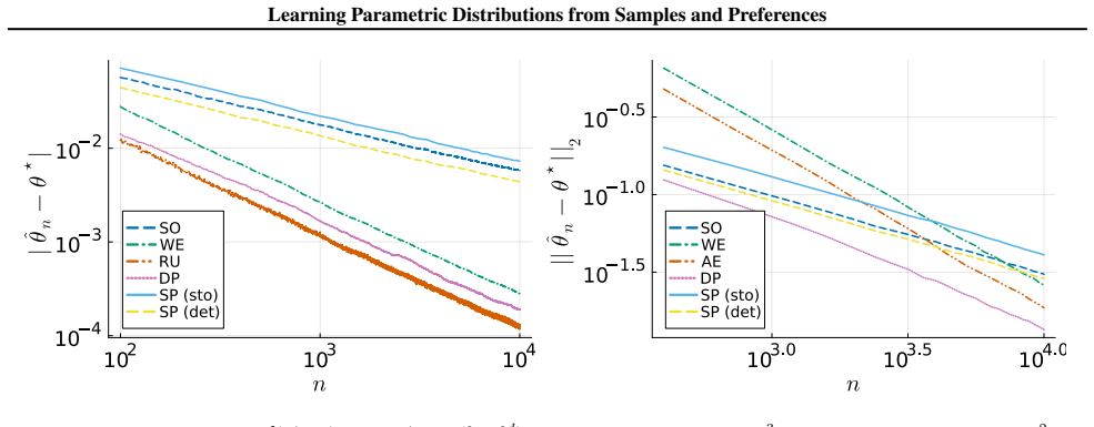
The central claim is that deterministic preference feedback changes the rate class of parametric estimation, not merely its constants. Under Assumptions 4.2, 4.4, 4.5 and 4.7, the paper proves that the diameter of the feasible set $C_n = \{\theta \in \Theta : Z_i \ell_\theta(X_i, Y_i) \ge 0 \;\forall i\}$ satisfies $\max_{\theta \in C_n} \|\theta - \theta^\star\| = O(1/n)$ with high probability. For Laplace and Gaussian families with log-probability rewards this yields $n|\hat\theta - \theta^\star| = O(\log(1/\delta))$ in one dimension, and for multivariate Gaussians $n\|\hat\theta - \theta^\star\|_\Sigma = O(A_d \log(1/\delta)\log n)$ with $A_d = O(\sqrt{d})$, so both the arbitrary feasible-set estimator and the deterministic-preferences MLE inherit the accelerated rate. Theorem 5.3 shows the rate cannot be improved: the minimax error is $\Omega(\min\{\alpha_F(k)\sqrt{k}/n, \sqrt{k/n}\})$, matching the upper bound up to dimension and problem-dependent constants. The mechanism is the same one that gives the sample-only uniform-location estimator its $\Theta(1/n)$ rate — a positive density crossing at the boundary of the constraint set — but now applied to constraints that cut through the interior of the parameter space, and the paper shows this is absent for stochastic preferences, which only improve asymptotic variance.

Load-bearing premise

The entire $O(1/n)$ acceleration rests on the assumption that, in every direction of the parameter space, the preference-scaled gap variable has a strictly positive density at zero, meaning there is always a positive chance of drawing a sample pair whose preference constraint cuts arbitrarily close to the true parameter; if that density were zero in any direction, the feasible set would shrink more slowly and the speed-up would degrade toward the $1/\sqrt{n}$ rate.

Editorial extensions

If this is right

Any estimator confined to $C_n$ — the arbitrary feasible-set estimator and the deterministic-preferences MLE — inherits the $O(1/n)$ error bound, so the acceleration is a property of the constraint set itself, not of a particular fitting algorithm.
For Gaussian means, DP MLE is never worse than sample-only MLE at any sample size (Lemma 4.1), and empirically it is the only estimator whose error tracks $\min\{d^{3/2}/n, \sqrt{d/n}\}$ as the dimension grows.
The accelerated rate is minimax: even with full knowledge of the preference mechanism, no estimator can beat order $1/n$ up to dimension and problem-dependent constants (Theorem 5.3).
Stochastic preferences buy only a mild variance reduction — quantified as a covariance gap near 0.17 for 1-D Gaussians — while deterministic preferences change the rate class, because only the latter produce hard constraints.
The assumptions, while restrictive, are verified for the Gaussian and Laplace families with log-probability rewards, giving explicit constants $A_{\theta^\star} = 2b$ for Laplace and $A_{\theta^\star} = O(\sqrt{d})$ for Gaussian.

Reading between the lines

Editorial extensions of the paper, not claims the author makes directly.

Beyond the paper: the same positive-density-at-zero mechanism should transfer to any feedback oracle that emits exact hard constraints, such as margin or threshold queries on rewards, so the $O(1/n)$ rate is likely a property of perfect binary constraints rather than of log-probability rewards specifically; the paper's margin example for Gaussian preferences already points in this direction.
Beyond the paper: the negative example of reference-anchored rewards ($\tilde\ell_\theta = \ell_\theta - \ell_{\theta_0}$) violates the informativeness assumption along the direction $\theta^\star - \theta_0$, suggesting that alignment objectives which subtract a frozen reference model discard exactly the directional preference information needed for fast estimation.
Beyond the paper: the Gaussian dimensionality gap — upper bound $O(A_{\theta^\star} d/n)$ versus lower bound $\Omega(\alpha_F(d)\sqrt{d}/n)$ — is the paper's stated open problem; analyzing the inradius rather than the diameter of the random polytope $C_n$ is a plausible route, since the worst-case directions may be statistically rare.

Share X Bluesky LinkedIn Reddit HN

Editorial analysis

A structured set of objections, weighed in public.

Desk editor's note, referee report, and a circularity audit.

Desk Editor's Note

read the letter

Marc, here is the one thing to know before you invest a weekend: this paper has a genuinely interesting fixed-dimension result, and a multivariate claim that does not survive contact with its own lower bound. The O(1/n) rate for deterministic preferences in fixed dimension is real and new, and the proof structure is honest and detailed. But Theorem 4.3, as stated for Gaussian d>1, contradicts Theorem 5.3 on dimension dependence. Theorem 4.3 gives n||theta_hat - theta*|| <= O(sqrt(d) log n); Theorem 5.3 with alpha_F(d)=A_theta*=O(sqrt(d)) gives a lower bound Omega(min{d/n, sqrt(d/n)}) = Omega(1) at n=d, while the claimed upper bound is o(1). The general covering bound in Theorem 4.8 only yields O(d^{3/2}/n), which is consistent with the lower bound. So the headline multivariate rate needs revision, either to eO(d^{3/2}/n) or explicitly to fixed d.

Credit where due: the core mechanism—hard constraints from deterministic preferences shrink the feasible set at rate 1/n via minima of positive-density variables—is well explained, with explicit assumptions, verified examples, a matching lower bound via Assouad, and code. That is reproducible work, and the appendices read carefully.

Soft spots, roughly in order: (1) the dimensional contradiction above; (2) the abstract's O(1/n) hides log n and dimension factors; (3) the claim that SPdet beats SP for multivariate Gaussian rests on an unproven conjecture on R^SPdet, supported only by numerics; (4) experiments lack error bars and use only 100 runs for d=20. Assumption 4.7 (positive density at zero) is genuinely restrictive, but the authors flag it themselves and give examples.

For fixed d, the central claim is likely correct and worth citing. The paper deserves a serious referee, but not in this form: the multivariate theorem needs to be corrected, not just caveated. I would send it back for major revision.

Referee Report

3 major / 4 minor

Summary. The paper studies estimation of a parameter theta of a continuous parametric family when the learner observes i.i.d. pairs (X_i,Y_i) drawn from p_theta* together with deterministic or stochastic preference labels Z_i generated from a parametric preference function. The main results are: (i) the stochastic-preference MLE has Fisher information I(p)+Delta, hence a smaller asymptotic variance than the sample-only MLE, and deterministic preferences improve this further; (ii) with deterministic preferences, the empirical 0-1 feasible set C_n yields estimators (arbitrary estimators and the DP MLE) with estimation error O(1/n) under explicit geometric assumptions; and (iii) a minimax lower bound Omega(1/n) via Assouad's lemma. The assumptions are verified for Gaussian and Laplace families with log-probability rewards, and experiments illustrate the rates.

Significance. The fixed-dimension O(1/n) rate for deterministic preference feedback is a genuinely interesting phenomenon, and the proof route through the minimum of positive random variables is clean and well documented. The paper ships detailed appendices with the main proofs, explicit constants for the Gaussian and Laplace examples, and reproducible code, which are notable strengths. The significance would be high if the statements are brought into full agreement with the proofs, because the result provides a clear parametric example in which preference feedback changes the convergence rate rather than only the asymptotic constant. However, as detailed below, the multivariate form of the headline upper bound is not supported by the general theorem and is inconsistent with the paper's own lower bound, so the central claim needs repair before the paper is publishable in its current form.

major comments (3)

[Section 4, Theorem 4.3] The multivariate statement n||theta_hat - theta*||_Sigma <= O(A_d log(1/delta) log n) with A_d = O(sqrt(d)), i.e. an error O(sqrt(d) log n / n), contradicts Theorem 5.3. Using the Gaussian computation alpha_F(d) = A_theta* = O(sqrt(d)) from Appendix F, Theorem 5.3 gives R_max >= Omega(min{d/n, sqrt(d/n)}) = Omega(d/n) whenever n >= c d. Taking n = d yields a lower bound Omega(1), while the claimed upper bound is O(log d / sqrt(d)) -> 0 as d -> infinity. The general covering argument in Theorem 4.8, optimized as described in the paragraph after the theorem, gives eO(A_theta* d/n) = O(d^{3/2}/n) for the Gaussian family, and the positive-examples paragraph after Theorem 4.8 states exactly this rate. Thus Theorem 4.3 is not a direct corollary of Theorem 4.8 as written, and its dimension dependence must be corrected; the fixed-d O(1/n) claim survives through Theorem 4.8.
[Section 5 and abstract] The abstract and Section 1 describe the lower bound as matching the upper bound, but the stated bounds do not match in dimension. Theorem 5.3 yields Omega(alpha_F(k) sqrt(k)/n), while Theorem 4.8 yields O(A_theta* k/n) after optimizing the covering radius; for the Gaussian case alpha_F(d) = A_theta* = O(sqrt(d)), so the lower bound is Omega(d/n) and the strongest upper bound from Theorem 4.8 is O(d^{3/2}/n). The paper explicitly acknowledges a dimensionality gap in the paragraph after Theorem 5.3, which is good, but the abstract's wording 'matching lower bound; up to dimension and problem-dependent constants' should be qualified to make clear that the match is in the exponent of n for fixed dimension, not in the dimension dependence.
[Appendix E, proof of Theorem 5.3] The proof of Theorem 5.3 begins by considering a hypercube Theta' = {theta_b = delta b : b in {0,1}^d} subseteq Theta. This requires Theta to contain a full cube of side length delta, but the problem statement only assumes Theta is bounded by B_Theta; no non-degeneracy condition guaranteeing the existence of such a cube is stated. If Theta is, for example, a low-dimensional subset of R^k, the displayed Assouad argument does not apply. This is fixable by adding an explicit assumption that Theta contains such a hypercube, but as stated the lower bound's scope is not fully justified.

minor comments (4)

[Theorem 4.3] The condition 'for all n >= O(log(1/delta))' is an asymptotic condition inside a non-asymptotic theorem; it should be stated as n >= C log(1/delta) for an explicit constant C, with the eO variant for the multivariate case made similarly precise.
[Appendix G, Proof of Assumption 4.7] The displayed formula for F'_theta*,u(x) is written as 1/(2b)e^{-2epsilon/b}, mixing the variable x and the parameter epsilon; the derivative should be expressed consistently as a function of the argument of F_theta*,u.
[Section 6, Figure 1] The text says 'SP performs worse than SO MLE' while the figure caption and Section 3 distinguish SPdet from SP; please keep the labeling consistent so the reader knows whether the deterministic or stochastic estimator is being compared.
[Appendix F, Proof of Assumption 5.2] The chain of inequalities for fBC uses the identity e^{1/4||theta-theta*||^2} fBC = 2F_theta*,u(epsilon); the intermediate change of variables is correct, but the sign of the exponent in the displayed factor e^{1/4||...||^2} is easy to misread as e^{-1/4||...||^2}. A one-line clarification would help.

Circularity Check

0 steps flagged · score 0.0 of 10

No circularity: the O(1/n) rate is derived from explicit probabilistic and analytic bounds, not from assuming the target result.

full rationale

No load-bearing circular step was found. The accelerated O(1/n) upper bound follows from a direct geometric and probabilistic argument: Rn,u is bounded by the minimum of Vθ*,u(Xi,Yi), and Lemma 4.6 gives P(Rn,u > ε) ≤ exp(−nFθ*,u(ε)). Assumption 4.7 only imposes that the inverse c.d.f. of Vθ*,u is regular near zero, and the paper verifies this by explicit closed-form computation for Gaussian and Laplace families rather than by assuming the final error bound. The constants Aθ*, Bθ*, Cθ* are derived analytically from pθ and ℓθ, not fitted to data. The lower bound uses Assouad's lemma and Assumption 5.2, whose Gaussian and Laplace verifications are independent calculations. The paper contains no self-citation chain that carries the argument: references to Van der Vaart, Tsybakov, Wainwright, and Tang et al. are contextual or methodological, not load-bearing. The only notable concern is an internal dimension-dependence inconsistency between the O(sqrt(d) log n / n) claim in Theorem 4.3 and the O(d^{3/2}/n) rate stated after Theorem 4.8, which also conflicts with the lower bound in Theorem 5.3; however, this is a correctness or consistency defect, not equivalence-by-construction or fitted-input-as-prediction. The central O(1/n) claim for fixed dimension is supported by an independent argument and therefore is not circular.

Assumptions & free parameters 0 free parameters · 7 assumptions · 0 invented entities

The central results rest on a set of explicitly stated geometric assumptions (4.2, 4.4, 4.5, 4.7, 5.2) that are verified for Gaussian and Laplace families with log-probability rewards. No free parameters are fitted to data: the constants A_theta*, B_theta*, C_theta* are derived analytically. The paper introduces no new physical or model entities. The main theoretical machinery is standard M-estimation, empirical risk minimization, and minimax lower bound techniques.

assumptions (7)

standard math Standard regularity conditions on p_theta and l_theta (Van der Vaart Chapter 5): three-times differentiability, uniform integrability of derivatives, so that integrals and derivatives can be exchanged.
Invoked implicitly in Sections 2 and 3 for asymptotic normality and consistency of M-estimators, and in the proofs in Appendix C.
domain assumption The parameter space Theta is bounded with diameter B_Theta.
Stated in the problem setup (Section 2, 'Let B_Theta := max_{theta in Theta} ||theta||'), and used for covering numbers in Theorem 4.8.
domain assumption Assumption 4.2 (Identifiability): For all theta != theta*, m(theta) = P(D(theta*, theta)) > 0, where D(theta*, theta) is the disagreement set.
Ensures that the set of minimizers of the population 0-1 loss C(theta*) equals {theta*}, so that 0-1 loss based estimators are consistent. Verified for Gaussian and Laplace.
domain assumption Assumption 4.4 (Linearization validity): For all theta != theta*, the linearized disagreement set eD(theta*, theta) is contained in the true disagreement set D(theta*, theta).
This guarantees C_n subset of eC_n, allowing the linearized feasible set to be used as a safe upper bound. Verified for Gaussian (equality, since l is linear in theta) and for Laplace.
domain assumption Assumption 4.5 (Informative preferences): For every direction u, P(G_1(theta*, u)) > 0, where G_1(theta*, u) is the set of pairs whose preference is informative along u.
Ensures that preferences constrain every direction in the parameter space. Verified for Gaussian (probability 1/2) and Laplace (probability 1/4).
domain assumption Assumption 4.7 (Positive density at zero and inverse CDF regularity): F'_{theta*,u}(0) in (0, inf) and a bound on the second derivative of the inverse CDF near zero.
This assumption provides the O(1/n) rate by making the inverse CDF of V_{theta*,u} scale linearly near zero. Verified with explicit constants for Laplace and via Lemma F.1 for Gaussian.
domain assumption Assumption 5.2 (Lower-bound regularity): There are constants c1, c2 and scaling alpha_F(k) such that fBC(tilde_theta, theta) + H^2(p_tilde_theta^2, p_theta^2) <= (c1/alpha_F(k)) ||theta - tilde_theta|| + c2 ||theta - tilde_theta||^2.
Needed to apply Assouad's lemma in Theorem 5.3 through Hellinger/TV bounds. Verified for Gaussian and Laplace in Appendices F and G.

how reviews work

0 comments

Cite this review

Pith. "Pith review of Learning Parametric Distributions from Samples and Preferences." pith.science (2026). https://pith.science/paper/STOWLRU6

@misc{pith2026250523557,
  author       = {Pith},
  title        = {Pith review of: Learning Parametric Distributions from Samples and Preferences},
  year         = {2026},
  howpublished = {\url{https://pith.science/paper/STOWLRU6}},
  note         = {Machine review of arXiv:2505.23557}
}

abstract

Recent advances in language modeling have underscored the role of preference feedback in enhancing model performance. This paper investigates the conditions under which preference feedback improves parameter estimation in classes of continuous parametric distributions. In our framework, the learner observes pairs of samples from an unknown distribution along with their relative preferences depending on the same unknown parameter. We show that preference-based M-estimators achieve a better asymptotic variance than sample-only M-estimators, further improved by deterministic preferences. Leveraging the hard constraints revealed by deterministic preferences, we propose an estimator achieving an estimation error scaling of $\mathcal{O}(1/n)$ -- a significant improvement over the $\Theta(1/\sqrt{n})$ rate attainable with samples alone. Next, we establish a lower bound that matches this accelerated rate; up to dimension and problem-dependent constants. While the assumptions underpinning our analysis are restrictive, they are satisfied by notable cases such as Gaussian or Laplace distributions for preferences based on the log-probability reward.

Figures

Figures reproduced from arXiv: 2505.23557 by the authors.

**Figure 1.** Estimation errors for N (θ ⋆ , Id) where θ ⋆ ∼ U([1, 2]d ) for (a) d = 1 with Nruns = 103 , and (b) d = 20 with Nruns = 102 . Theorem 5.3. Let Rmax := infθb supθ ⋆∈Θ Eqθ⋆ [∥θb− θ ⋆∥]. Suppose Assumption 5.2 holds. Then, Rmax ≥ Ω [PITH_FULL_IMAGE:figures/full_fig_p008_1.png] view at source ↗

**Figure 2.** Estimation errors as a function of d with N (θ ⋆ , Id) where θ ⋆ ∼ U([1, 2]d ), for n = 104 and Nruns = 103 . This further highlights the weakness of asymptotic results compared to non-asymptotic guarantees. While [PITH_FULL_IMAGE:figures/full_fig_p009_2.png] view at source ↗

**Figure 3.** Approximations of ∆SP N(0d,Id) , ∆ SPdet N(0d,Id) and R SPdet N(0d,Id) by (a) αdId and (b) associated error for varying d. Nruns = 106 . Proof that Pp ⊗2 θ⋆ (G1(θ ⋆ )) > 0. It is direct to see that dim(G0(θ ⋆ ) ∁ ) < 2d and dim(G0(θ ⋆ ) \ G1(θ ⋆ )) < 2d. Given that p ⊗2 θ ⋆ is a continuous distribution on (R d ) 2 , we obtain that Pp ⊗2 θ⋆ (G1(θ ⋆ )) = Pp ⊗2 θ⋆ (G0(θ ⋆ )) = 1. Condition in Lemma 3.1. The condition o… view at source ↗

Figures from the paper (5 more)

**Figure 4.** Figure 4: Estimation errors for (a) Lap(θ ⋆ , 1) where θ ⋆ ∼ U([1, 2]) with Nruns = 10 and (b) Rayleigh( √ θ ⋆) where θ ⋆ ∼ U([1, 2]) with Nruns = 102 . The estimators based on Cn are θbAE n ∈ Cn, θbWE n := arg maxθ∈Cn |θ − θ ⋆ | and θbDP n = arg max θ∈Cn X i∈[n] (|Yi − θ| + |Xi…

**Figure 5.** Figure 5: Estimation errors for N (θ ⋆ , Id) where θ ⋆ ∼ U([1, 2]d ) with Nruns = 102 for (a) d = 1 and (b) d = 20. Proof of Assumption 4.4 and 4.5. Since ℓθ(x, y) = (x 2 − y 2 )θ + log(x/y) is linear in θ, we have D(θ ⋆ , θ) = De(θ ⋆ , θ). Let (X, Y ) ∼ p ⊗2 θ ⋆ . Then, we have…

**Figure 6.** Figure 6: Estimation errors as a function of d with N (θ ⋆ , Id) where θ ⋆ ∼ U([1, 2]d ), for n = 104 and Nruns = 102 . Multivariate Gaussian. For d > 1, multiple centers exist. We use the Chebyshev center estimator (CCE) of Cn. Figures 5(b) and 6 shows that CCE outperforms AE b…

**Figure 7.** Figure 7: (a) [PITH_FULL_IMAGE:figures/full_fig_p028_7.png]

**Figure 8.** Figure 8: Estimation errors when minimizing the empirical losses for N (θ ⋆ , 1) where θ ⋆ ∼ U([1, 2]) with Nruns = 102 when (a) normalizing by β with regularization λ = 1 and (b) regularizing by λ with normalization β = 1. Figures 8(a) and (b) showcase the “mild” impact of norm…

Discussion (0). Sign in to comment.

Reference graph

Works this paper leans on

19 extracted references · 8 canonical work pages

[5]

local” Assumptions 4.2 and 4.4 are satisfied. Given that Assumption 4.4 is based on “ignoring

• In Appendix F, for FN,Σ and preferences based on rθ = logp θ, we prove all the assumptions introduced in this paper. • In Appendix G, for FLap,b and preferences based on rθ = logp θ, we prove all the assumptions introduced in this paper. • In Appendix H, we provide supplementary experiments to support our theoretical findings. B. Extended Discussions We...

work page 2024
[7]

J., Rohatgi, D., Zhang, C., Simchowitz, M., Ash, J

Huang, A., Block, A., Foster, D. J., Rohatgi, D., Zhang, C., Simchowitz, M., Ash, J. T., and Krishnamurthy, A. Self-improvement in language models: The sharpening mechanism. InNeurIPS 2024 Workshop on Mathematics of Modern Machine Learning,

work page 2024
[10]

S., and Bag- nell, J

Swamy, G., Choudhury, S., Sun, W., Wu, Z. S., and Bag- nell, J. A. All roads lead to likelihood: The value of reinforcement learning in fine-tuning.arXiv preprint arXiv:2503.01067,

arXiv
[15]

M., Stiennon, N., Wu, J., Brown, T

Ziegler, D. M., Stiennon, N., Wu, J., Brown, T. B., Radford, A., Amodei, D., Christiano, P., and Irving, G. Fine-tuning language models from human preferences.arXiv preprint arXiv:1909.08593,

arXiv 1909
[17]

reversed

and ASFT (Wang et al., 2024), see, e.g., Gorbatovski et al. (2025). Without separability, solving Eq. (5) can be NP-hard. Under sufficient regularity, bθDP n converges to θ0 ∈arg min θ∈Θ{KL(θ⋆, θ) +λm(θ)}where 13 Learning Parametric Distributions from Samples and Preferences m(θ) =P p⊗2 θ⋆ (D(θ⋆, θ))and θ0 ̸=θ ⋆. As θ7→m(θ) can be non-convex, computing θ0...

work page 2025
[18]

Let ε=θ−θ ⋆

We consider the case θ⋆ < θsince θ⋆ > θis done similarly as fBC(θ⋆, θ) =fBC(θ, θ⋆). Let ε=θ−θ ⋆. By integrating for x < y, we have fBC(θ⋆, θ) = 1 2b2 Z x ex/b Z y 1(x≤θ ⋆ <(x+y)/2< θ ⋆ +ε≤y)e −y/bdy dx + e−(ε+θ⋆)/b 2b2 Z x ex/b Z y 1(y < θ⋆ +ε∧x≤θ ⋆ <(x+y)/2) dy dx + e−ε/b 2b2 Z x Z y 1(θ ⋆ < x < y < θ⋆ +ε) dy dx + e−θ⋆/b 2b2 Z y e−y/b Z x 1(θ ⋆ < x∧(x+y)...

work page 2017
[102]

spiky” along some directions. Due to those distant vertices, the center would become a worse estimator than DP, since the “average

Multivariate Gaussian.Ford >1, multiple centers exist. We use the Chebyshev center estimator (CCE) ofC n. Figures 5(b) and 6 shows that CCE outperforms AE by a constant margin. It only outperforms DP in the regime of large n compared to d and performs worse than SO MLE for small n. Geometrically, for small n and large d, we conjecture that the random poly...

work page 2024
[1946]

The llama 3 herd of models.arXiv preprint arXiv:2407.21783,

Dubey, A., Jauhri, A., Pandey, A., Kadian, A., Al-Dahle, A., Letman, A., Mathur, A., Schelten, A., Yang, A., Fan, A., et al. The llama 3 herd of models.arXiv preprint arXiv:2407.21783,

arXiv

Show all 19 references

[1952]

Gorbatovski, A., Shaposhnikov, B., Sinii, V ., Malakhov, A., and Gavrilov, D

doi: 10.1002/j.1538-7305.1952.tb01393.x. Gorbatovski, A., Shaposhnikov, B., Sinii, V ., Malakhov, A., and Gavrilov, D. The differences between di- rect alignment algorithms are a blur.arXiv preprint arXiv:2502.01237,

1952
[2012]

Ge, L., Juba, B., and V orobeychik, Y

doi: 10.1137/120865094. Ge, L., Juba, B., and V orobeychik, Y . Learning linear util- ity functions from pairwise comparison queries.arXiv preprint arXiv:2405.02612,

arXiv
[2013]

Leveraging sparsity for sample-efficient preference learning: A theoretical per- spective.arXiv preprint arXiv:2501.18282,

Yao, Y ., He, L., and Gastpar, M. Leveraging sparsity for sample-efficient preference learning: A theoretical per- spective.arXiv preprint arXiv:2501.18282,

arXiv
[2014]

Orpo: Monolithic prefer- ence optimization without reference model

Hong, J., Lee, N., and Thorne, J. Orpo: Monolithic prefer- ence optimization without reference model. InProceed- ings of the 2024 Conference on Empirical Methods in Natural Language Processing, pp. 11170–11189,

2024
[2017]

URL https://epubs.siam.org/ doi/10.1137/141000671

doi: 10.1137/ 141000671. URL https://epubs.siam.org/ doi/10.1137/141000671. Birgé, L. and Massart, P. Rates of convergence for mini- mum contrast estimators.Probability Theory and Related Fields, 97:113–150,

doi
[2019]

Asft: Aligned supervised fine-tuning through absolute likelihood.arXiv preprint arXiv:2409.10571,

Wang, R., Sun, J., Hua, S., and Fang, Q. Asft: Aligned supervised fine-tuning through absolute likelihood.arXiv preprint arXiv:2409.10571,

arXiv
[2020]

URL http://dx.doi.org/10.1145/3372885

doi: 10.1145/3372885.3373824. URL http://dx.doi.org/10.1145/3372885. 3373824. Meng, Y ., Xia, M., and Chen, D. Simpo: Simple preference optimization with a reference-free reward.Advances in Neural Information Processing Systems, 37:124198– 124235,
[2022]

Touvron, H., Martin, L., Stone, K., Albert, P., Almahairi, A., Babaei, Y ., Bashlykov, N., Batra, S., Bhargava, P., Bhosale, S., et al

https://www.sagemath.org. Touvron, H., Martin, L., Stone, K., Albert, P., Almahairi, A., Babaei, Y ., Bashlykov, N., Batra, S., Bhargava, P., Bhosale, S., et al. Llama 2: Open foundation and fine- tuned chat models.arXiv preprint arXiv:2307.09288,

arXiv
[2023]

Proximal policy optimization algorithms

Schulman, J., Wolski, F., Dhariwal, P., Radford, A., and Klimov, O. Proximal policy optimization algorithms. arXiv preprint arXiv:1707.06347,

arXiv
[2024]

Constitutional ai: Harmlessness from ai feedback.arXiv preprint arXiv:2212.08073,

Bai, Y ., Kadavath, S., Kundu, S., Askell, A., Kernion, J., Jones, A., Chen, A., Goldie, A., Mirhoseini, A., McKin- non, C., et al. Constitutional ai: Harmlessness from ai feedback.arXiv preprint arXiv:2212.08073,

arXiv
[2025]

D., Zheng, Z., Calandriello, D., Munos, R., Rowland, M., Richemond, P

Tang, Y ., Guo, Z. D., Zheng, Z., Calandriello, D., Munos, R., Rowland, M., Richemond, P. H., Valko, M., Avila Pires, B., and Piot, B. Generalized preference optimization: A unified approach to offline alignment. In Salakhutdinov, R., Kolter, Z., Heller, K., Weller, A., Oliver...

arXiv

Pith tools

Reviewed August 7, 2026 · model on record in the stance chip above.

[1] [5]

local” Assumptions 4.2 and 4.4 are satisfied. Given that Assumption 4.4 is based on “ignoring

• In Appendix F, for FN,Σ and preferences based on rθ = logp θ, we prove all the assumptions introduced in this paper. • In Appendix G, for FLap,b and preferences based on rθ = logp θ, we prove all the assumptions introduced in this paper. • In Appendix H, we provide supplementary experiments to support our theoretical findings. B. Extended Discussions We...

work page 2024

[2] [7]

J., Rohatgi, D., Zhang, C., Simchowitz, M., Ash, J

Huang, A., Block, A., Foster, D. J., Rohatgi, D., Zhang, C., Simchowitz, M., Ash, J. T., and Krishnamurthy, A. Self-improvement in language models: The sharpening mechanism. InNeurIPS 2024 Workshop on Mathematics of Modern Machine Learning,

work page 2024

[3] [10]

S., and Bag- nell, J

Swamy, G., Choudhury, S., Sun, W., Wu, Z. S., and Bag- nell, J. A. All roads lead to likelihood: The value of reinforcement learning in fine-tuning.arXiv preprint arXiv:2503.01067,

arXiv

[4] [15]

M., Stiennon, N., Wu, J., Brown, T

Ziegler, D. M., Stiennon, N., Wu, J., Brown, T. B., Radford, A., Amodei, D., Christiano, P., and Irving, G. Fine-tuning language models from human preferences.arXiv preprint arXiv:1909.08593,

arXiv 1909

[5] [17]

reversed

and ASFT (Wang et al., 2024), see, e.g., Gorbatovski et al. (2025). Without separability, solving Eq. (5) can be NP-hard. Under sufficient regularity, bθDP n converges to θ0 ∈arg min θ∈Θ{KL(θ⋆, θ) +λm(θ)}where 13 Learning Parametric Distributions from Samples and Preferences m(θ) =P p⊗2 θ⋆ (D(θ⋆, θ))and θ0 ̸=θ ⋆. As θ7→m(θ) can be non-convex, computing θ0...

work page 2025

[6] [18]

Let ε=θ−θ ⋆

We consider the case θ⋆ < θsince θ⋆ > θis done similarly as fBC(θ⋆, θ) =fBC(θ, θ⋆). Let ε=θ−θ ⋆. By integrating for x < y, we have fBC(θ⋆, θ) = 1 2b2 Z x ex/b Z y 1(x≤θ ⋆ <(x+y)/2< θ ⋆ +ε≤y)e −y/bdy dx + e−(ε+θ⋆)/b 2b2 Z x ex/b Z y 1(y < θ⋆ +ε∧x≤θ ⋆ <(x+y)/2) dy dx + e−ε/b 2b2 Z x Z y 1(θ ⋆ < x < y < θ⋆ +ε) dy dx + e−θ⋆/b 2b2 Z y e−y/b Z x 1(θ ⋆ < x∧(x+y)...

work page 2017

[7] [102]

spiky” along some directions. Due to those distant vertices, the center would become a worse estimator than DP, since the “average

Multivariate Gaussian.Ford >1, multiple centers exist. We use the Chebyshev center estimator (CCE) ofC n. Figures 5(b) and 6 shows that CCE outperforms AE by a constant margin. It only outperforms DP in the regime of large n compared to d and performs worse than SO MLE for small n. Geometrically, for small n and large d, we conjecture that the random poly...

work page 2024

[8] [1946]

The llama 3 herd of models.arXiv preprint arXiv:2407.21783,

Dubey, A., Jauhri, A., Pandey, A., Kadian, A., Al-Dahle, A., Letman, A., Mathur, A., Schelten, A., Yang, A., Fan, A., et al. The llama 3 herd of models.arXiv preprint arXiv:2407.21783,

arXiv