REVIEW 4 major objections 5 minor 39 references
3-D Positioning and Environment Mapping for mmWave Communication Systems
T0 review · 4 major / 5 minor · reviewed 2026-08-14 · deepseek-v4-flash
Pith's one-line read A closed-form weighted least-squares estimator jointly locates and tracks a moving mmWave user from hybrid TDoA/FDoA/AoA measurements and maps surrounding walls from single-bounce reflections, with a neural-network variant reaching…
desk verdict A solid closed-form WLS estimator for 3D mmWave localization and mapping, but the SLAM validation is circular and the velocity results rely on synthetic FDoA. read the letter →
The pith
A machine-rendered reading of the paper's core claim, the machinery that carries it, and where it could break.
The reading
What carries the argument
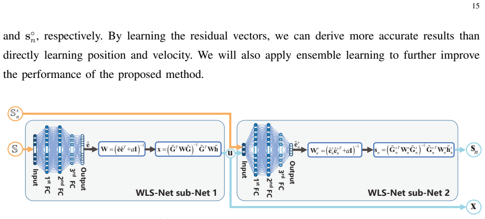
The load-bearing mechanism is pseudo-linearization plus weighted least squares. By squaring the TDoA range equations and rewriting the angle equations with the unit vectors $a_n=(\cos\theta_n\cos\phi_n,\cos\theta_n\sin\phi_n,\sin\theta_n)^T$, $c_n=(-\sin\phi_n,\cos\phi_n,0)^T$, and $d_n=(-\sin\theta_n\cos\phi_n,-\sin\theta_n\sin\phi_n,\cos\theta_n)^T$, the unknown position and velocity enter linearly, giving pseudo-linear equations $h=Gx^\circ$. A weighting matrix $W=(B Q B^T)^{-1}$ is derived from the first-order propagation of measurement noise through the equations and is updated iteratively; this choice is what makes the estimator approach the Cramér-Rao lower bound. In WLS-Net, a fully connected network learns the residual $e$ itself, so the weighting matrix can be built from the learned residual plus a small regularization term, removing the need for a known $Q$ and for iterations.
What would settle it
Run the environment-mapping algorithm on ray-tracing scenes that include known double-bounce reflectors and check whether estimated scatterer positions land on real walls; or independently classify the second- and third-strongest paths in the public ray-tracing dataset from ground-truth ray-interaction data and count how many are actually single-bounce rather than assumed to be.
Extended reading notes
Core claim
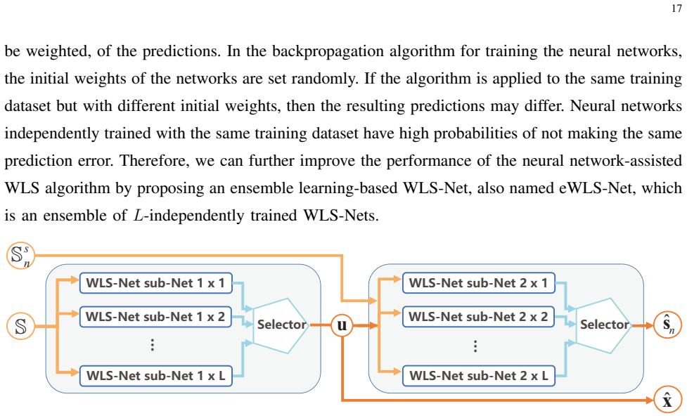
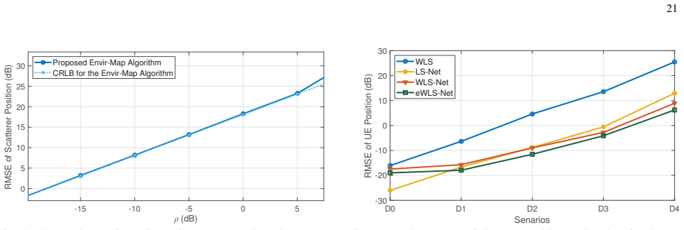
The paper's central claim is that a single-stage closed-form WLS solution can solve the joint position/velocity and environment-mapping problems in 3-D mmWave CRANs. From the nonlinear geometry, the authors build pseudo-linear systems $h=Gx^\circ$ and $h_n^s=G_n^s s_n^\circ$ by squaring range equations and exploiting the unit direction vectors of the angle measurements. The estimator $x=(\tilde G^T W \tilde G)^{-1}\tilde G^T W \tilde h$, with $W=(B Q B^T)^{-1}$ where $B$ linearizes the measurement-error propagation, is proven asymptotically unbiased (Theorem 1) and is shown to attain the CRLB under low Gaussian noise (Theorem 2); the same construction is applied to scatterer mapping. The paper further claims that replacing the linear approximation with a neural network that learns the residual vector $e$, then using $W=(\hat e \hat e^T + a I)^{-1}$, improves accuracy when measurement errors are correlated, and that ensembling $L$ independently trained WLS-Nets with a subtractive-clustering selector gives the best results. On the ray-tracing dataset, the reported numbers are centimeter-level user-position RMSE (0.0104 m for eWLS-Net) while the pure WLS gives 0.02 m.
Load-bearing premise
Every mapped reflection is a single bounce off one point-like surface in the environment, and the second and third strongest paths in the ray-tracing data really are such single-bounce paths; if a measured path bounces twice, spreads diffusely, or has higher-order interactions, the reconstructed wall locations stop being meaningful.
Editorial extensions
If this is right
- With three or more LoS-connected RRHs, the one-stage WLS outperforms the downlink single-bounce reference scheme, and using two RRHs already matches its accuracy.
- In the low-noise regime the joint estimator reaches the CRLB for position and velocity; as measurement noise grows, the performance deviates only slowly.
- The environment-mapping WLS reaches the CRLB for scatterer position, so walls and other reflectors can be reconstructed from single-bounce NLoS paths without specular-reflection assumptions or prior UE position and direction.
- WLS-Net and eWLS-Net run without iterations and without knowing the noise covariance, cutting runtime to about 18-21% of the iterative WLS while improving accuracy when measurement errors are correlated.
Reading between the lines
- Editorial inference: residual learning should also help when measurement errors carry systematic, position-dependent biases (for example antenna misalignment or clock-drift leftovers), because those are the conditions under which the paper's correlated-error experiments show the largest gains.
- Editorial inference: since WLS-Net does not need the noise covariance matrix $Q$, a natural next step is training on simulated residual statistics and deploying in a new environment without per-site noise calibration; the paper does not test cross-scene transfer.
- Editorial inference: the single-bounce assumption is the fragile point, so a practical SLAM system built on this method would need a separate path-order classifier to reject double-bounce, diffuse, and higher-order multipath before mapping; the paper does not provide such a classifier.
Signed reviews
Editorial analysis
A structured set of objections, weighed in public.
Referee Report
Summary. The paper considers 3-D joint position and velocity estimation and environment mapping in a millimeter-wave cloud radio access network. It formulates hybrid TDoA/FDoA/AoA measurements, derives a closed-form weighted least squares (WLS) estimator for the user position/velocity, proves asymptotic unbiasedness and CRLB attainment under a first-order noise approximation, and extends the approach to single-bounce NLoS scatterer mapping with a second WLS estimator. It then introduces WLS-Net and ensemble eWLS-Net, which learn the residual error vectors instead of the position directly, and evaluates them on a public ray-tracing dataset (DeepMIMO/Remcom). The numerical sections report decimeter-level accuracy for the WLS estimator, CRLB-consistent Monte Carlo curves, and centimeter-level position accuracy for eWLS-Net on the ray-tracing dataset.
Significance. If the results hold, the paper makes a useful contribution by providing a one-stage closed-form WLS solution for 3-D joint position/velocity estimation from hybrid measurements, with an explicit CRLB comparison and Monte Carlo validation. The neural-network-assisted extension is a sensible way to combine geometric models with learned residuals, and the use of a public ray-tracing dataset is a strength. The derivations in Appendices A–D are detailed and the CRLB-matching behavior at low noise is convincingly demonstrated for the joint position/velocity estimator. However, the environment-mapping and SLAM claims are currently supported by a CRLB that ignores the propagation of UE position error, and by a single-bounce assumption whose validation is circular; these issues must be addressed before the environment-mapping claims can be accepted.
major comments (4)
- [Section IV and Fig. 8] The environment-mapping CRLB comparison treats the UE position u° as exactly known when constructing h_s^n and G_s^n in (41), but in practice the scatterer estimator (44) is evaluated with the UE position estimate from Algorithm 1, and Algorithm 2 explicitly states that it uses "the UE position u° obtained in Algorithm 1." The error in u propagates into the scatterer estimate, and the RMSE of the mapping is therefore bounded by a joint CRLB that includes the UE position uncertainty, not by the conditional CRLB plotted in Fig. 8. The text in Section VI-B acknowledges that "the position estimation error of the UE will then proceed to the proposed environment mapping algorithm," but the CRLB curve does not incorporate this effect. The claim that the mapping algorithm "can achieve the CRLB" is therefore overstated; the authors should either derive the joint CRLB or explicitly present the current curve as a conditional CRLB for a known UE position.
- [Section VI-B, Fig. 7] The validation of the single-bounce NLoS assumption is circular. The paper states that "most of the second and third strongest paths in the ray-tracing dataset are verified to be the single-bounce NLoS paths" based on the observation that the scatterer positions estimated by the proposed algorithm "match the position of the walls." However, the environment-mapping estimator in Section IV is constrained to place each scatterer on the measured AoA ray at a distance determined by the round-trip delay under the single-bounce model. A double-bounce or higher-order path can also produce a point on a building facade that satisfies these geometric constraints, so wall matching does not distinguish single-bounce paths from higher-order paths. An independent path-order audit using the ray-tracing ground truth (e.g., labeling paths by number of interactions in Remcom) or a quantitative comparison of predicted single-bounce delays against the measured delays is needed. This issue is load-bearing because the environment-mapping estimator, WLS-Net sub-Net 2, and the SLAM results in Table II all inherit the single-bounce assumption.
- [Section VI-C, Table II] The FDoA measurements used in the ray-tracing experiments are not part of the public dataset; the paper states that "There are no FDoA measurements given in the ray-tracing dataset. For each user, we generate its speed in a random way, and then calculate its corresponding FDoA measurements." Consequently, the velocity RMSE entries in Table II (v = 0.0143, 0.0054, 0.0039 m/s) are not validated against the ray-tracing data but against a synthetic measurement model with randomly generated speeds. The "centimeter-level accuracy" claim is a position-only claim, and the velocity performance should be presented as a synthetic-data result, not as a property of the ray-tracing dataset. This limitation should be stated explicitly wherever the Table II results are summarized.
- [Section III-C, Theorem 1 and Remark 1] Theorem 1 states that the estimator is "asymptotically unbiased," and Remark 1 explains this as meaning that "the proposed algorithm will become increasingly accurate as the number of measurements increases." The proof, however, shows only that E{Δx} ≈ 0 under the first-order approximation E{e} ≈ B E{Δm} = 0, which is an approximate unbiasedness for small Gaussian noise, not an asymptotic property in the number of measurements. If consistency as N_a grows is intended, a different argument is required; as written, the theorem and the remark do not match the proof. The statement should be revised to "approximately unbiased under small measurement noise" or a proper asymptotic analysis should be provided.
minor comments (5)
- [Algorithm 2, line 2] Algorithm 2 says "the UE position u° obtained in Algorithm 1," but u° denotes the true value elsewhere in the paper; the algorithm actually uses the estimate u from Algorithm 1. Rename the variable to u or u_hat to avoid confusion.
- [Section VI-B, Fig. 8] The RMSE curves in Figs. 5–9 are plotted in dB, but the axis labels do not specify the reference value (e.g., dB relative to 1 m or 1 m/s). Adding the reference would make the figures self-contained.
- [Notations] In the Notations section, "|c| denotes the module of c" should read "modulus of c."
- [Section VI-C] The paper introduces a "dominant fixed error" component in the D0–D4 scenarios, but the theoretical analysis in Section III-C assumes a zero-mean Gaussian noise vector with covariance Q. Clarify that the WLS optimality and CRLB analysis apply to the Gaussian random part, while the neural-network methods are designed to also learn the fixed part.
- [Section V-A, Eq. (46)] The regularization constant a in W = (ê ê^T + aI)^{-1} is described only as "a very small disturbance value," but no value is reported in the numerical section. Please state the chosen value and its sensitivity, since it affects the WLS-Net results.
Circularity Check
Closed-loop validation of the single-bounce assumption; the WLS/CRLB core derivation is independent.
-
other
[Section VI-B, Fig. 7 (environment mapping with the ray-tracing dataset); Algorithm 2 and Eq. (33)]
"The estimated locations of the scatterers match the position of the walls of the buildings ... Second, most of the second and third strongest paths in the ray-tracing dataset are verified to be the single-bounce NLoS paths, which also corroborates the assumption of the proposed environment mapping algorithm."
The verification uses scatterer positions estimated by the proposed environment-mapping WLS solver (Algorithm 2), whose model (33)-(39) is derived from the single-bounce relation d1 + d2 = r_s + r_1. For a double-bounce or higher-order path, this solver still returns the point on the measured AoA ray whose round-trip distance equals the measured delay, and that point can lie on a building wall behind the first reflection point. Therefore, wall-matching of the estimated points is a consistency check of the single-bounce model with itself, not an independent path-order audit.
full rationale
The load-bearing statistical derivations are not circular. The WLS joint position/velocity estimator (Section III) is derived from noise-free pseudo-linear equations, and its asymptotic unbiasedness and CRLB attainment (Theorems 1 and 2) are proven against an externally defined CRLB (Eq. 22) using first-order perturbation of the measurement noise; the Monte Carlo comparisons in Section VI-A provide an independent numerical check. The WLS-Net/eWLS-Net results are evaluated on held-out samples from an external ray-tracing dataset, so the learned residual vectors are not fitted to the test targets. The one genuine circular element is the validation of the single-bounce NLoS assumption in Section VI-B: the environment-mapping algorithm that is used to produce the scatterer positions already assumes single-bounce, and those estimated positions are then used to claim that the dataset paths are indeed single-bounce. This does not invalidate the WLS estimation theory, but it means the environment-mapping/SLAM credibility currently rests on a partially self-confirming consistency check rather than on independent evidence of path order.
Assumptions & free parameters
free parameters (3)
- a (WLS-Net regularization constant) =
not specified
- ra and rb (subtractive clustering radii) =
not specified
- L (ensemble size) =
10
assumptions (7)
- domain assumption Only LoS and single-bounce NLoS paths exist in the mmWave channel, and each RRH-UE pair has at most one scatterer for the model.
- domain assumption The LoS path is stronger than NLoS paths and can be selected via a threshold, so Na LoS RRHs are known.
- domain assumption Measurement noise is a zero-mean Gaussian vector with known covariance Q, and similarly Qs_n for mapping.
- domain assumption The error vector e is well approximated by the first-order term B Delta m.
- domain assumption The UE position estimate from Algorithm 1 is treated as exact when mapping scatterers and when computing the environment-mapping CRLB.
- domain assumption Scatterers are static point reflectors and the environment is stationary during estimation.
- ad hoc to paper The second and third strongest paths in the ray-tracing dataset correspond to single-bounce NLoS paths.
Cite this review
Pith. "Pith review of 3-D Positioning and Environment Mapping for mmWave Communication Systems." pith.science (2026). https://pith.science/paper/SUY3ELIB
@misc{pith2026190804142,
  author       = {Pith},
  title        = {Pith review of: 3-D Positioning and Environment Mapping for mmWave Communication Systems},
  year         = {2026},
  howpublished = {\url{https://pith.science/paper/SUY3ELIB}},
  note         = {Machine review of arXiv:1908.04142}
}
read the original abstract
Millimeter-wave (mmWave) cloud radio access networks (CRANs) provide new opportunities for accurate cooperative localization, in which large bandwidths, large antenna arrays, and increased densities of base stations allow for their unparalleled delay and angular resolution. Combining localization into communications and designing simultaneous localization and mapping (SLAM) algorithms are challenging problems. This study considers the joint position and velocity estimation and environment mapping problem in a three-dimensional mmWave CRAN architecture. We first embed cooperative localization into communications and establish the joint estimation and mapping model with hybrid delay and angle measurements. Then, we propose a closed-form weighted least square (WLS) solution for the joint estimation and mapping problems. The proposed WLS estimator is proven asymptotically unbiased and confirmed by simulations as effective in achieving the Cramer-Rao lower bound (CRLB) and the desired decimeter-level accuracy. Furthermore, we propose a WLS-Net-based SLAM algorithm by embedding neural networks into the proposed WLS estimators to replace the linear approximations. The solution possesses both powerful learning ability of the neural network and robustness of the proposed geometric model, and the ensemble learning is applied to further improve positioning accuracy. A public ray-tracing dataset is used in the simulations to test the performance of the WLS-Net-based SLAM algorithm, which is proven fast and effective in attaining the centimeter-level accuracy.
Figures

Figures from the paper (3 more)


Reference graph
Works this paper leans on
-
[1]
Massive MIMO is a Reality -- What is Next? Five Promising Research Directions for Antenna Arrays
E. Bj ¨ornson, L. Sanguinetti, H. Wymeersch, J. Hoydis, and T. L. Marzetta, “Massive MIMO is a reality-what is next? Five promising research directions for antenna arrays,” https://arxiv.org/abs/1902.07678
work page Pith review arXiv 1902
-
[2]
Localization as a feature of mmWave communication,
F. Lemic, J. Martin, C. Yarp, D. Chan, V . Handziski, R. Brodersen, G. Fettweis, A. Wolisz, and J. Wawrzynek, “Localization as a feature of mmWave communication,” in Proc. IEEE IWCMC , Sep. 2016, pp. 1033-1038
work page 2016
-
[3]
Survey of cellular mobile radio localization methods: From 1G to 5G,
J. A. del Peral-Rosado, R. Raulefs, J. A. L ´opez-Salcedo, and G. Seco-Granados, “Survey of cellular mobile radio localization methods: From 1G to 5G,” IEEE Commun. Surv. Tutor., vol. 20, no. 2, pp. 1124-1148, May 2018
work page 2018
-
[4]
5G mmWave positioning for vehicular networks,
H. Wymeersch, G. Seco-Granados, G. Destino, D. Dardari, and F. Tufvesson, “5G mmWave positioning for vehicular networks,” IEEE Wireless Commun. Mag. , vol. 24, no. 6, pp. 80-86, Dec. 2017
work page 2017
-
[5]
An overview of signal processing techniques for millimeter wave MIMO systems,
R. W. Heath, Jr., N. G. Prelcic, S. Rangan, W. Roh, and A. Sayeed, “An overview of signal processing techniques for millimeter wave MIMO systems,” IEEE J. Sel. Top. Signal Process. , vol. 10, no. 3, pp. 436-453, Apr. 2016
work page 2016
-
[6]
Investigation of transmission schemes for millimeter-wave massive MU-MIMO systems,
Y . Han, H. Zhang, S. Jin, X. Li, R. Yu, and Y . Zhang, “Investigation of transmission schemes for millimeter-wave massive MU-MIMO systems,” IEEE Syst. J. , vol. 11, no. 1, pp. 72-83, Mar. 2017
work page 2017
-
[7]
Mm-wave MIMO channel modeling and user localization using sparse beamspace signatures,
H. Deng and A. M. Sayeed, “Mm-wave MIMO channel modeling and user localization using sparse beamspace signatures,” in Proc. IEEE SPAWC, Jun. 2014, pp. 130-134
work page 2014
-
[8]
Beamspace channel estimation in mmWave systems via cosparse image reconstruction technique,
J. Yang, C. K. Wen, S. Jin, and F. Gao, “Beamspace channel estimation in mmWave systems via cosparse image reconstruction technique,” IEEE Trans. Commun. , vol. 66, no. 10, pp. 4767-4782, Oct. 2018
work page 2018
Show all 39 references
-
[9]
Uplink channel estimation and data transmission in millimeter-wave CRAN with lens antenna arrays,
R. G. Stephen and R. Zhang, “Uplink channel estimation and data transmission in millimeter-wave CRAN with lens antenna arrays,” IEEE Trans. Commun. , vol. 66, no. 12, pp. 6542-6555, Jul. 2018
2018
-
[10]
Location-aware communications for 5G networks: How location information can improve scalability, latency, and robustness of 5G,
R. D. Taranto, S. Muppirisetty, R. Raulefs, D. Slock, T. Svensson, and H. Wymeersch, “Location-aware communications for 5G networks: How location information can improve scalability, latency, and robustness of 5G,” IEEE Signal Process. Mag. , vol. 31, no. 6, pp. 102-112, Nov. 2014
2014
-
[11]
A survey on 5G massive MIMO localization,
F. Wen, H. Wymeersch, B. Peng, W. P. Tay, H. C. So, and D. Yang, “A survey on 5G massive MIMO localization,” Digit. Signal Process, 2019, https://doi.org/10.1016/j.dsp.2019.05.005
2019 doi
-
[12]
Positioning via direct localization in C-RAN systems,
S. Jeong, O. Simeone, A. Haimovich, and J. Kang, “Positioning via direct localization in C-RAN systems,” IET Commun. , vol. 10, no. 16, pp. 2238-2244, Jun. 2016
2016
-
[13]
Direct localization for massive MIMO,
N. Garcia, H. Wymeersch, E. G. Larsson, A. M. Haimovich, and M. Coulon, “Direct localization for massive MIMO,” IEEE Trans. Signal Process., vol. 65, no. 10, pp. 2475-2487, May 2017
2017
-
[14]
Weighted least squares algorithm for target localization in distributed MIMO radar,
M. Einemo and H. C. So, “Weighted least squares algorithm for target localization in distributed MIMO radar,” Signal Process., vol. 115, no. C, pp. 144-150, Oct. 2015
2015
-
[15]
Asymptotically efficient target localization from bistatic range measurements in distributed MIMO radars,
R. Amiri, F. Behnia, and H. Zamani, “Asymptotically efficient target localization from bistatic range measurements in distributed MIMO radars,” IEEE Signal Process. Lett. , vol. 24, no. 3, pp. 299-303, Jan. 2017
2017
-
[16]
An asymptotically efficient estimator in closed-form for 3-D AOA localization using a sensor network,
Y . Wang and K. C. Ho, “An asymptotically efficient estimator in closed-form for 3-D AOA localization using a sensor network,” IEEE Trans. Wireless Commun. , vol. 14, no. 12, pp. 6524-6535, Jul. 2015
2015
-
[17]
Efficient 3-D positioning using time-delay and AoA measurements in MIMO radar systems,
R. Amiri, F. Behnia, and H. Zamani, “Efficient 3-D positioning using time-delay and AoA measurements in MIMO radar systems,” IEEE Commun. Lett. , vol. 21, no. 12, pp. 2614-2617, Aug. 2017
2017
-
[18]
An accurate algebraic solution for moving source location using TDoA and FDoA measurements,
K. C. Ho and W. W. Xu, “An accurate algebraic solution for moving source location using TDoA and FDoA measurements,” IEEE Trans. Signal Process. , vol. 52, no. 9, pp. 2453-2463, Aug. 2004
2004
-
[19]
Multistatic pseudolinear target motion analysis using hybrid measurements,
N. H. Nguyen and K. Dogancay, “Multistatic pseudolinear target motion analysis using hybrid measurements,” Signal Process., vol. 130, no. C, pp. 22-36, Jan. 2017
2017
-
[20]
5G mmWave downlink vehicular positioning,
H. Wymeersch, N. Garcia, H. Kim, G. Seco-Granados, S. Kim, F. Wen, and M. Fr ¨ohle, “5G mmWave downlink vehicular positioning,” in Proc. IEEE GLOBECOM , Dec. 2018, pp. 1-6
2018
-
[21]
Efficient multisensor localization for the internet of things: Exploring a new class of scalable localization algorithms,
M. Z. Win, F. Meyer, Z. Liu, W. Dai, S. Bartoletti, and A. Conti, “Efficient multisensor localization for the internet of things: Exploring a new class of scalable localization algorithms,” IEEE Signal Process. Mag. vol. 35, no. 5, pp. 153-167, Sept. 2018
2018
-
[22]
Distributed localization: A linear theory,
S. Safavi, U. A. Khan, S. Kar, and J. M. F. Moura, “Distributed localization: A linear theory,” Proc. IEEE, vol. 106, no. 7, pp. 1204-1223, Jul. 2018. 30
2018
-
[23]
Nonline-of-sight error mitigation in mobile location,
L. Cong and W. Zhuang, “Nonline-of-sight error mitigation in mobile location,” IEEE Trans. Wireless Commun. , vol. 4, no. 2, pp. 560-573, Mar. 2005
2005
-
[24]
A survey on TOA based wireless localization and NLOS mitigation techniques,
I. Guvenc and C.-C. Chong, “A survey on TOA based wireless localization and NLOS mitigation techniques,” IEEE Commun. Surv. Tutor., vol. 11, no. 3, pp. 107-124, Aug. 2009
2009
-
[25]
High-accuracy localization for assisted living: 5G systems will turn multipath channels from foe to friend,
K. Witrisal et al., “High-accuracy localization for assisted living: 5G systems will turn multipath channels from foe to friend,” IEEE Signal Process. Mag. , vol. 33, no. 2, pp. 59-70, Mar. 2016
2016
-
[26]
Simultaneous localization and mapping: Part I,
H. Durrant-Whyte and T. Bailey, “Simultaneous localization and mapping: Part I,” IEEE Robot. Autom. Mag. , vol. 13, no. 2, pp. 99-110, Jun. 2006
2006
-
[27]
Leveraging mmWave imaging and communications for simultaneous localization and mapping,
M. Aladsani, A. Alkhateeb, and G. C. Trichopoulos, “Leveraging mmWave imaging and communications for simultaneous localization and mapping,” in Proc. IEEE ICASSP , May. 2019, pp. 4539-4543
2019
-
[28]
Multipath assisted positioning with simultaneous localization and mapping,
C. Gentner, T. Jost, W. Wang, S. Zhang, A. Dammann, and U. Fiebig, “Multipath assisted positioning with simultaneous localization and mapping,” IEEE Trans. Wireless Commun. , vol. 15, no. 9, pp. 6104-6117, Sept. 2016
2016
-
[29]
Millimeter wave channel modeling and cellular capacity evaluation,
M. R. Akdeniz et al., “Millimeter wave channel modeling and cellular capacity evaluation,” IEEE J. Sel. Areas Commun. , vol. 32, no. 6, pp. 1164-1179, Jun. 2014
2014
-
[30]
38GHz and 60GHz angle-dependent propagation for cellular & peer-to-peer wireless communications,
T. S. Rappaport, E. Ben-Dor, J. N. Murdock, and Y . Qiao, “38GHz and 60GHz angle-dependent propagation for cellular & peer-to-peer wireless communications,” in Proc. IEEE ICC , Jun. 2012, pp. 4568-4573
2012
-
[31]
DeepFi: Deep learning for indoor fingerprinting using channel state information,
X. Wang, L. Gao, S. Mao, and S. Pandey, “DeepFi: Deep learning for indoor fingerprinting using channel state information,” in Proc. IEEE WCNC , Mar. 2015, pp. 1666-1671
2015
-
[32]
CSI-based outdoor localization for massive MIMO: Experiments with a learning approach,
A. Decurninge, L. G. Ord ´o˜nez, P. Ferrand, G. He, B. Li, W. Zhang, and M. Guillaud, “CSI-based outdoor localization for massive MIMO: Experiments with a learning approach,” in Proc. IEEE ISWCS , Aug. 2018, pp. 1-6
2018
-
[33]
DeepMIMO: A generic deep learning dataset for millimeter wave and massive MIMO applications,
A. Alkhateeb, “DeepMIMO: A generic deep learning dataset for millimeter wave and massive MIMO applications,” in Proc. IEEE ITA, Feb. 2019, pp. 1-8
2019
-
[34]
Wireless insite,
Remcom, “Wireless insite,” http://www.remcom.com/wireless-insite
-
[35]
Channel estimation in broadband millimeter wave MIMO systems with few-bit ADCs,
J. Mo, P. Schniter, and R. W. Heath. Jr, “Channel estimation in broadband millimeter wave MIMO systems with few-bit ADCs,” IEEE Trans. Signal Process. , vol. 66, no. 5, pp. 1141-1154, Jan. 2018
2018
-
[36]
Initial access in milllimeter wave cellular systems,
C. N. Barati et al., “Initial access in milllimeter wave cellular systems,” IEEE Trans. Wireless Commun. , vol. 15, no. 12, pp. 7926-7940, Dec. 2016
2016
-
[37]
S. M. Kay, Fundamentals of statistical signal processing, Estimation Theory. Englewood Cliffs, NJ, USA: Prentice-Hall, 1993
1993
-
[38]
T. G. Dietterich, Ensemble learning, The handbook of brain theory and neural networks. Cambridge, MA: MIT Press, 2002
2002
-
[39]
Towards optimal power control via ensembling deep learning neural networks,
F. Liang, C. Shen, W. Yu, and F. Wu, “Towards optimal power control via ensembling deep learning neural networks,” https://arxiv.org/abs/1807.10025
Reviewed August 14, 2026 · model on record in the stance chip above.
Discussion (0). Continue with ORCID to comment.