Recovering Sharp Conductivity Features in the Finite-Data Calder\'on Problem with Physics-Informed Neural Networks
Pith reviewed 2026-06-29 04:43 UTC · model grok-4.3
The pith
Physics-informed neural networks recover dominant conductivity structures from finite boundary measurements with 3-12% relative error.
A machine-rendered reading of the paper's core claim, the machinery that carries it, and where it could break.
Core claim
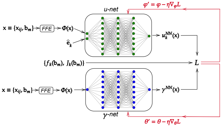
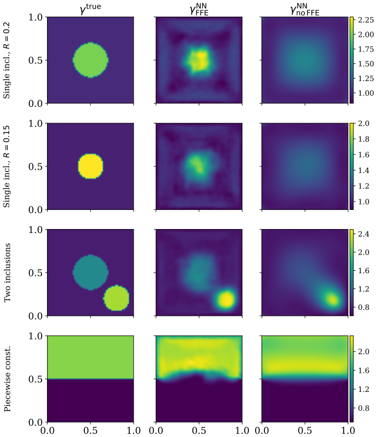
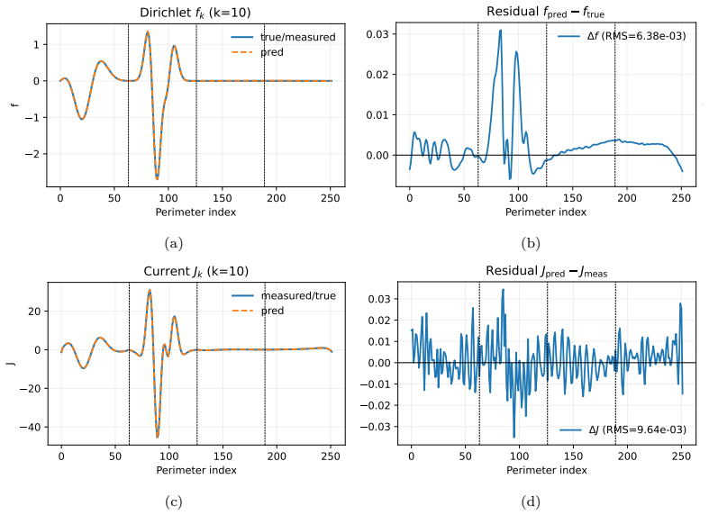
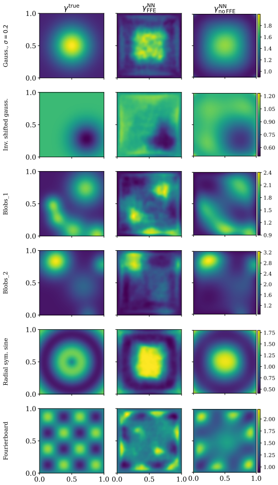
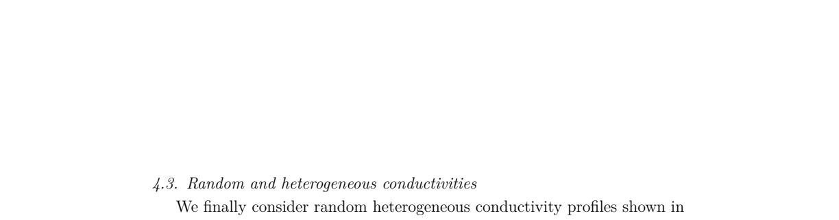
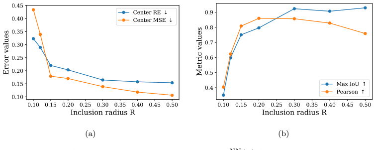
The central claim is that representing conductivity and potentials with separate neural networks conditioned on randomized wavelet boundary excitations, then minimizing a physics-informed loss that combines elliptic PDE residuals with finite boundary DtN losses, reconstructs conductivity fields containing inclusions, sharp interfaces, smooth profiles, and heterogeneous media from limited data, with relative errors of 3% to 12%. Fourier feature encoding improves recovery of localized sharp features while raw-coordinate networks remain competitive for smoother fields.
What carries the argument
Separate neural networks for conductivity and the family of electric potentials, conditioned on boundary excitations, with physics-informed residuals enforcing the elliptic conductivity equation and Fourier feature encoding to represent sharp spatial variations.
If this is right
- Fourier feature encoding improves reconstruction of localized sharp features such as inclusions and interfaces.
- Raw-coordinate networks perform competitively when the conductivity field is smoother.
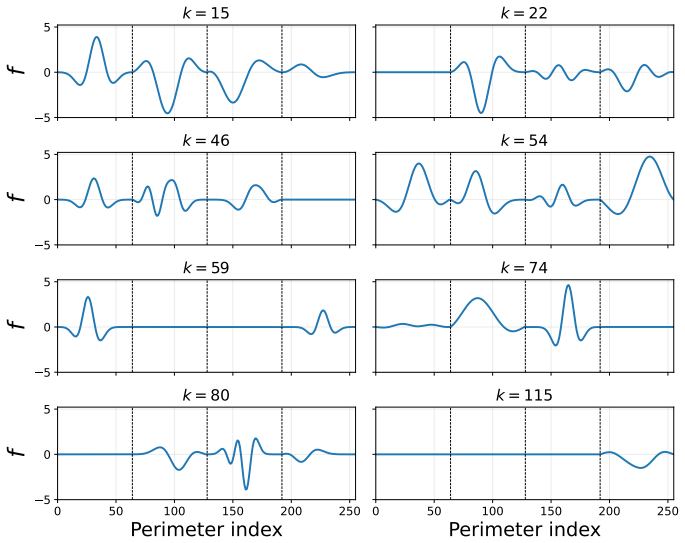
- Multiscale wavelet boundary excitations enable recovery of dominant structures from limited data.
- The framework applies to conductivity fields that include both sharp and smooth components.
Where Pith is reading between the lines
- The relative performance of Fourier versus raw encodings indicates that input representation choice is critical when neural networks approximate discontinuous inverse-problem solutions.
- The same separation of conductivity and potential networks could be tested on other elliptic inverse problems that supply only partial boundary maps.
- If the synthetic-data assumption holds in practice, the method supplies a route to hybrid physics-ML solvers for electrical impedance tomography.
Load-bearing premise
The synthetic data generated by the finite-difference forward solver provides an accurate representation of the finite Dirichlet-to-Neumann map for the elliptic conductivity problem.
What would settle it
Reconstructing a known conductivity field from boundary data generated by a different numerical solver or from laboratory measurements and checking whether the relative error stays inside the reported 3-12% range.
Figures
read the original abstract
Physics-informed neural networks (PINNs) have recently emerged as a promising framework for addressing the Calder\'on inverse problem from limited boundary data. In this work, we revisit neural Calder\'on inversion by introducing multiscale boundary excitations based on randomized wavelet functions and investigating the role of Fourier-feature encoding (FFE) for representing sharp conductivity variations. We propose a physics-informed reconstruction framework that represents the unknown conductivity and the associated family of electric potentials with separate neural networks conditioned on the applied boundary excitations. The governing elliptic PDE is enforced through physics-informed residuals, while finite Dirichlet-to-Neumann (DtN) data are incorporated through boundary losses. Using synthetic data from a finite-difference forward solver, we evaluate the method on conductivity fields with inclusions, sharp interfaces, smooth profiles, and heterogeneous media. Results show that the framework recovers dominant conductivity structures from finite boundary measurements with relative errors between $3\%-12\%$ approximately. We show that FFE improves the reconstruction of localized sharp features, particularly for inclusions and interfaces, but are not universally optimal, with raw-coordinate networks performing competitively for smoother fields. These results highlight coordinate representations and boundary excitation design as key factors in neural Calder\'on inversion.
Editorial analysis
A structured set of objections, weighed in public.
Referee Report
Summary. The paper introduces a PINN framework for the Calderón inverse problem that represents conductivity and electric potentials with separate networks conditioned on boundary excitations. It employs randomized wavelet-based multiscale excitations, enforces the elliptic PDE via physics residuals, and matches finite DtN data through boundary losses. Synthetic data from a finite-difference solver is used to test recovery on inclusions, sharp interfaces, smooth profiles, and heterogeneous media, claiming 3–12% relative errors with FFE aiding localized sharp features (though not universally optimal).
Significance. If the central empirical claims hold after addressing discretization consistency, the work would provide concrete evidence that coordinate representations and excitation design matter for neural Calderón inversion on limited boundary data. The tests across multiple conductivity classes and the observation that raw-coordinate networks can compete for smooth fields are useful empirical contributions.
major comments (1)
- [§3 (data generation) and §2.2 (loss)] The evaluation uses boundary data generated by a finite-difference forward solver while the physics-informed loss enforces the continuous elliptic conductivity PDE. This mismatch is especially relevant near discontinuities, where FD truncation and numerical diffusion are absent from the residual; the reported improvement from FFE on sharp inclusions and interfaces may therefore partly reflect fitting of discrete artifacts rather than genuine recovery of the continuous inverse problem. (See data-generation paragraph in §3 and the residual formulation in §2.2.)
minor comments (2)
- [Abstract and §4] The abstract states relative errors of 3%–12% without error bars, baseline comparisons, or details on data exclusion / hyperparameter sensitivity; these should be added to the results section for reproducibility.
- [§2.1] Notation for the family of potentials and the conditioning on excitations is introduced without an explicit equation reference; a single clarifying equation would improve readability.
Simulated Author's Rebuttal
We thank the referee for the constructive comment highlighting the discretization consistency issue. We address it directly below and outline targeted revisions.
read point-by-point responses
-
Referee: [§3 (data generation) and §2.2 (loss)] The evaluation uses boundary data generated by a finite-difference forward solver while the physics-informed loss enforces the continuous elliptic conductivity PDE. This mismatch is especially relevant near discontinuities, where FD truncation and numerical diffusion are absent from the residual; the reported improvement from FFE on sharp inclusions and interfaces may therefore partly reflect fitting of discrete artifacts rather than genuine recovery of the continuous inverse problem. (See data-generation paragraph in §3 and the residual formulation in §2.2.)
Authors: We acknowledge the discretization mismatch between the finite-difference forward solver (used to generate synthetic DtN data) and the continuous elliptic PDE residual in the PINN loss. This is a valid concern, especially near discontinuities where FD numerical diffusion may introduce artifacts not present in the continuous model. The finite-difference solver is a conventional choice for synthetic data in Calderón problem studies, and sufficiently refined grids provide a reasonable approximation; however, it does not eliminate the inconsistency. Regarding FFE, while it may partially interact with discrete effects, the empirical pattern—that FFE aids sharp inclusions/interfaces while raw coordinates compete for smooth fields—suggests it primarily enhances representation capacity rather than solely fitting artifacts. In the revision we will (i) expand the data-generation paragraph in §3 to explicitly discuss the FD approximation and its limitations, (ii) add a brief limitations paragraph noting the mismatch and suggesting future consistent discretizations (e.g., finite-element or spectral forward models), and (iii) include a short grid-resolution sensitivity remark if space allows. These changes clarify the scope without altering the core empirical claims. revision: partial
Circularity Check
No significant circularity; empirical PINN inversion on independent synthetic data
full rationale
The paper implements a standard PINN setup for the Calderón problem: separate networks for conductivity and potentials, physics residuals enforcing the elliptic PDE, and boundary losses matching finite DtN data generated by an external finite-difference solver. Reported 3-12% relative errors are direct numerical outcomes on test fields (inclusions, interfaces, smooth profiles). No derivation step reduces by construction to its inputs, no fitted parameters are relabeled as predictions, and no load-bearing self-citations or uniqueness theorems from prior author work are invoked. The method is self-contained against the provided synthetic benchmarks.
Axiom & Free-Parameter Ledger
free parameters (2)
- Fourier feature mapping parameters
- Wavelet scale and randomization parameters
axioms (2)
- domain assumption The electric potential satisfies the conductivity equation ∇ · (σ ∇ u) = 0 inside the domain
- domain assumption Separate neural networks conditioned on boundary excitations can represent the conductivity and the associated family of potentials
Reference graph
Works this paper leans on
-
[1]
A. P. Calderón, On an inverse boundary value problem, Computational & Applied Mathematics 25 (2-3) (2006) 133–138.(Reprinted from: Seminar on numerical analysis and its applications to continuum physics (1980)). URLhttps://www.scielo.br/j/cam/a/fr8pXpGLSmDt8JyZyxvfwbv/
2006
-
[2]
J. Sylvester, G. Uhlmann, A global uniqueness theorem for an inverse boundary value problem, Annals of Mathematics 125 (1) (1987) 153–169. URLhttp://www.jstor.org/stable/1971291
-
[3]
Alessandrini, Stable determination of conductivity by boundary mea- surements, Applicable Analysis 27 (1988) 153–172
G. Alessandrini, Stable determination of conductivity by boundary mea- surements, Applicable Analysis 27 (1988) 153–172. URLhttps://api.semanticscholar.org/CorpusID:120037778
1988
-
[4]
J. L. Mueller, S. Siltanen, The d-bar method for electrical impedance tomography–demystified, Inverse Problems 36 (9) (2020) 093001.doi: 10.1088/1361-6420/aba2f5
-
[5]
Raissi, P
M. Raissi, P. Perdikaris, G. Karniadakis, Physics-informed neural net- works: A deep learning framework for solving forward and inverse prob- lems involving nonlinear partial differential equations, Journal of Compu- tational Physics 378 (2019) 686–707.doi:https://doi.org/10.1016/ j.jcp.2018.10.045
2019
-
[6]
L. Yang, X. Meng, G. E. Karniadakis, B-pinns: Bayesian physics- informed neural networks for forward and inverse pde problems with noisy data, Journal of Computational Physics 425 (2021) 109913
2021
-
[7]
Y. Bea, R. Jimenez, D. Mateos, S. Liu, P. Protopapas, P. Tarancón- Álvarez, P. Tejerina-Pérez, Gravitational duals from equations of state, JHEP 07 (2024) 087.arXiv:2403.14763, doi:10.1007/JHEP07(2024) 087
-
[8]
P. Tarancón-Álvarez, P. Tejerina-Pérez, R. Jimenez, P. Protopapas, Efficient pinns via multi-head unimodular regularization of the solutions space, Communications Physics 8 (1) (2025) 335.doi:https://doi. org/10.1038/s42005-025-02248-1. 31
-
[9]
L. Bar, N. Sochen, Strong solutions for pde-based tomography by un- supervised learning, SIAM Journal on Imaging Sciences 14 (1) (2021) 128–155
2021
-
[10]
Pokkunuru, P
A. Pokkunuru, P. Rooshenas, T. Strauss, A. Abhishek, T. Khan, Im- proved training of physics-informed neural networks using energy-based priors: a study on electrical impedance tomography, in: The eleventh international conference on learning representations, 2023
2023
-
[11]
Xuanxuan, Z
Y. Xuanxuan, Z. Yangming, C. Haofeng, M. Gang, W. Xiaojie, Cpfi-eit: A cnn-pinn framework for full-inverse electrical impedance tomography on non-smooth conductivity distributions, arXiv e-prints (2024) arXiv–2412
2024
-
[12]
J. Castro, C. Muñoz, N. Valenzuela, The calderón’s problem via deeponets, Vietnam Journal of Mathematics 52 (3) (2024) 775–806. doi:10.1007/s10013-023-00674-8
-
[13]
L. Lu, P. Jin, G. Pang, Z. Zhang, G. Karniadakis, Learning nonlinear operators via deeponet based on the universal approximation theorem of operators, Nature Machine Intelligence 3 (2021) 218–229.doi:10.1038/ s42256-021-00302-5
2021
-
[14]
R. Molinaro, Y. Yang, B. Engquist, S. Mishra, Neural inverse operators for solving pde inverse problems (2023).arXiv:2301.11167. URLhttps://arxiv.org/abs/2301.11167
-
[15]
Z. Li, N. Kovachki, K. Azizzadenesheli, B. Liu, K. Bhattacharya, A. Stu- art, A. Anandkumar, Fourier neural operator for parametric partial differential equations (2021).arXiv:2010.08895
work page internal anchor Pith review Pith/arXiv arXiv 2021
-
[16]
Rahaman, A
N. Rahaman, A. Baratin, D. Arpit, F. Draxler, M. Lin, F. Hamprecht, Y. Bengio, A. Courville, On the spectral bias of neural networks, in: K. Chaudhuri, R. Salakhutdinov (Eds.), Proceedings of the 36th Inter- national Conference on Machine Learning, Vol. 97 of Proceedings of Machine Learning Research, PMLR, 2019, pp. 5301–5310. URLhttps://proceedings.mlr.p...
2019
-
[17]
G. Uhlmann, Electrical impedance tomography and calderón’s problem, Inverse Problems 25 (12) (2009) 123011.doi:10.1088/0266-5611/25/ 12/123011. 32
-
[18]
A. I. Nachman, Global uniqueness for a two-dimensional inverse boundary value problem, Annals of Mathematics 143 (1) (1996) 71–96. doi: 10.2307/2118653
-
[19]
Astala, L
K. Astala, L. Päivärinta, Calderón’s inverse conductivity problem in the plane, Annals of Mathematics 163 (1) (2006) 265–299.doi:10.4007/ annals.2006.163.265
2006
-
[20]
P. CARO, K. M. ROGERS, Global uniqueness for the calderÓn problem with lipschitz conductivities, Forum of Mathematics, Pi 4 (2016) e2. doi:10.1017/fmp.2015.9
-
[21]
N. Mandache, Exponential instability in an inverse problem for the Schrödinger equation, Inverse Problems 17 (5) (2001) 1435–1444.doi: 10.1088/0266-5611/17/5/313
-
[22]
G. Alessandrini, Open issues of stability for the inverse conductivity problem, Journal of Inverse and Ill-posed Problems 15 (5) (2007) 451–460. doi:doi:10.1515/jiip.2007.025
-
[23]
M. W. M. G. Dissanayake, N. Phan-Thien, Neural-network-based approx- imations for solving partial differential equations, Communications in Nu- merical Methods in Engineering 10 (3) (1994) 195–201.arXiv:https:// onlinelibrary.wiley.com/doi/pdf/10.1002/cnm.1640100303, doi: https://doi.org/10.1002/cnm.1640100303
-
[24]
Artificial neural networks for solving ordinary and partial differential equations
I. Lagaris, A. Likas, D. Fotiadis, Artificial neural networks for solving ordinary and partial differential equations, IEEE Transactions on Neural Networks 9 (5) (1998) 987–1000.doi:10.1109/72.712178
-
[25]
J. Sirignano, K. Spiliopoulos, Dgm: A deep learning algorithm for solving partial differential equations, Journal of Computational Physics 375 (2018) 1339–1364.doi:10.1016/j.jcp.2018.08.029
-
[26]
Y. Zhu, N. Zabaras, L. Lu, P. Perdikaris, Physics-constrained deep learning for high-dimensional surrogate modeling and uncertainty quan- tification without labeled data, Journal of Computational Physics 394 (2019) 56–81.doi:10.1016/j.jcp.2019.05.024. 33
-
[27]
Mattheakis, P
M. Mattheakis, P. Protopapas, D. Sondak, M. D. Giovanni, E. Kaxiras, Physical symmetries embedded in neural networks (2020).arXiv:1904. 08991
2020
-
[28]
A. Choudhary, J. F. Lindner, E. G. Holliday, S. T. Miller, S. Sinha, W. L. Ditto, Physics-enhanced neural networks predict order and chaos, Physical Review E 101 (6) (2020) 062207.doi:10.1103/PhysRevE.101. 062207
-
[29]
A. Choudhary, J. F. Lindner, E. G. Holliday, S. T. Miller, S. Sinha, W. L. Ditto, Forecasting hamiltonian dynamics without canonical coordinates, arXiv preprint arXiv:2010.15201 (2020). doi:10.48550/arXiv.2010. 15201
-
[30]
S. Greydanus, M. Dzamba, J. Yosinski, Hamiltonian neural networks, arXiv preprint arXiv:1906.01563 (2019). doi:10.48550/arXiv.1906. 01563
-
[31]
G. E. Karniadakis, I. G. Kevrekidis, L. Lu, P. Perdikaris, S. Wang, L. Yang, Physics-informed machine learning, Nature Reviews Physics 3 (2021) 422–440.doi:10.1038/s42254-021-00314-5
-
[32]
C. Flamant, P. Protopapas, D. Sondak, Solving differential equations using neural network solution bundles (2020).arXiv:2006.14372
-
[33]
D. P. Kingma, J. Ba, Adam: A method for stochastic optimization (2017). arXiv:1412.6980. URLhttps://arxiv.org/abs/1412.6980
work page internal anchor Pith review Pith/arXiv arXiv 2017
-
[34]
Neural-network meth- ods for boundary value problems with irregular boundaries
I. Lagaris, A. Likas, D. Papageorgiou, Neural-network methods for boundary value problems with irregular boundaries, IEEE Transactions on Neural Networks 11 (5) (2000) 1041–1049.doi:10.1109/72.870037
-
[35]
Z. Wang, A. Bovik, H. Sheikh, E. Simoncelli, Image quality assessment: from error visibility to structural similarity, IEEE Transactions on Image Processing 13 (4) (2004) 600–612.doi:10.1109/TIP.2003.819861. 34 Appendix A. Finite Differences Method (FDM) forward solver To train and evaluate the aforementioned method, we generated synthetic boundary data b...
discussion (0)
Sign in with ORCID, Apple, or X to comment. Anyone can read and Pith papers without signing in.