REVIEW 2 major objections 6 minor 2 cited by
Priorconditioned Sparsity-Promoting Projection Methods for Deterministic and Bayesian Linear Inverse Problems
T0 review · 2 major / 6 minor · reviewed 2026-08-16 · deepseek-v4-flash
Pith's one-line read Priorconditioned Krylov subspaces solve sparsity-promoting IRLS in far fewer iterations, with better reconstructions, than existing S-GKS methods.
desk verdict Priorconditioning for sparsity-promoting GKS is a real contribution and the numerics are encouraging, but the main spectral proof has a genuine gap for rank-deficient Ψ and the paper needs revision, not desk rejection. read the letter →
The pith
A machine-rendered reading of the paper's core claim, the machinery that carries it, and where it could break.
The reading
What carries the argument
The load-bearing object is the oblique $A$-weighted pseudoinverse $(W_{\ell+1}\Psi)^{\dagger}_A = E(W_{\ell+1}\Psi)^{\dagger}$, where $E$ projects off the null space of $\Psi$; this is the standard-form transformation that converts each IRLS problem into Tikhonov regularization with an identity regularization operator. The argument is carried by the spectral bound in Theorem 4.3, which shows that the priorconditioned normal equations have at most $\operatorname{rank}(A)+1$ distinct eigenvalues clustered near $\mu$, making conjugate-gradient polynomial approximation effective. In practice, matvecs with this pseudoinverse are computed by an inner preconditioned conjugate-gradient method whose preconditioner is the unweighted, DCT-diagonalized pseudoinverse of $\Psi$.
What would settle it
On a small inverse problem where $(W\Psi)^{\dagger}_A$ can be formed exactly, run PS-GKS twice, once with exact pseudoinverse matvecs and once with the paper's DCT-preconditioned conjugate-gradient inner solver at practical tolerances, over a sequence of IRLS weights approaching zero. If iteration counts or final relative residual error diverge substantially, or if the computed spectrum of $Q^{\mathrm{pr}}_\mu$ violates the Theorem 4.3 bounds, the claimed acceleration rests on an inner solve the paper does not control rather than on priorconditioning itself.
Extended reading notes
Core claim
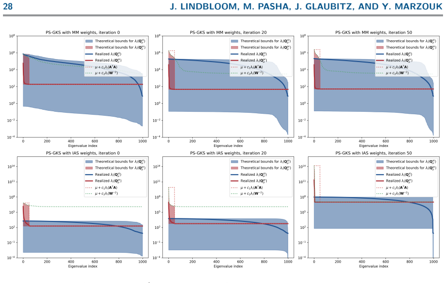
The paper's central discovery is that the priorconditioned normal equations $Q^{\mathrm{pr}}_\mu = \overline{A}^T\overline{A} + \mu I_K$, where $\overline{A} = A(W\Psi)^{\dagger}_A$, have a clustered spectrum. Theorem 4.3 shows that the $R$ nonzero eigenvalues satisfy $\mu \le \lambda_i(Q^{\mathrm{pr}}_\mu) \le \mu + \min\{c_1 \lambda_i(A^T A), c_2 \lambda_i(W^{-2})\}$ for $i = 1,\dots,R$, and that the remaining $K-R$ eigenvalues are all exactly $\mu$. Consequently the condition number of the priorconditioned system is bounded independently of the relative scaling of the IRLS weights, unlike the standard-form system, whose condition number blows up as the weights encode the sparsity pattern. The paper argues that this clustering is why PS-GKS converges in substantially fewer iterations and reaches sparser, more accurate reconstructions than S-GKS, and why restarted and recycled variants retain the gain under memory limits.
Load-bearing premise
The method assumes that at every outer iteration it can accurately apply the weighted oblique pseudoinverse of the sparsifying transform, even when the reweighting drives the weighted operator toward singularity; no accuracy or stability analysis is given for how accurate that inner computation must be.
Editorial extensions
If this is right
- Across both MM ($\ell_1$) and IAS (GSBL) weights, PS-GKS reaches lower relative residual error and higher SSIM and sparsity indices than S-GKS within the same iteration budget, and the theory predicts the gap widens as the weights promote sparsity more aggressively.
- Restarted and recycled variants, resPS-GKS and recPS-GKS, keep nearly the same reconstruction quality while capping the stored basis dimension, reducing memory and lowering the number of pseudoinverse matvecs.
- Within the IAS algorithm, the priorconditioned formulation enables automatic selection of the generalized gamma hyper-prior rate parameter through the discrepancy principle, eliminating manual fine-tuning of that parameter.
- The method works for rank-deficient sparsifying operators such as the anisotropic gradient used in the CT experiments, because the oblique pseudoinverse handles the null space of $\Psi$ without requiring $\Psi$ to be invertible.
- Priorconditioned variants are comparatively insensitive to the smoothing parameter $\varepsilon$ in the MM weights, so $\varepsilon$ can be chosen small without the instability that degrades S-GKS.
Reading between the lines
- Inference: because the spectral-clustering mechanism is a property of the priorconditioned operator rather than of generalized Krylov subspaces specifically, the same acceleration should transfer to Golub-Kahan and flexible Krylov IRLS solvers; the paper's own PS-GKB results already point in that direction.
- Inference: a natural testable extension is to derive an accuracy tolerance for the inner DCT-preconditioned conjugate-gradient solve that guarantees the outer spectral bounds still hold; without such a tolerance, near-zero IRLS weights may silently corrupt every outer iteration in large-scale use.
- Inference: the automatic rate-parameter selection likely extends to any scale-mixture-of-normals prior, including Laplace, horseshoe, and Besov priors, which would make hierarchical Bayesian edge-preserving inversion broadly less dependent on manual tuning.
Signed reviews
Editorial analysis
A structured set of objections, weighed in public.
Referee Report
Summary. The manuscript proposes PS-GKS, a priorconditioned generalized Krylov subspace method for solving the iteratively reweighted least-squares (IRLS) subproblems that arise in deterministic ℓ_p-regularization (via MM weights) and in hierarchical Bayesian GSBL estimation (via the IAS algorithm). The authors also introduce restarted and recycled variants (resPS-GKS, recPS-GKS) and a Golub–Kahan analogue (PS-GKB). The central claim is that priorconditioning substantially accelerates convergence and improves reconstruction quality relative to existing S-GKS, res/recS-GKS, FGK, and FLSQR methods, while also enabling automatic selection of the GSBL rate parameter. The paper includes a theoretical analysis (Theorems 4.2 and 4.3) intended to show that priorconditioning clusters the spectrum of the projected normal equations, and two numerical experiments: a 1D undersampled DCT problem and a 2D limited-angle CT problem with an anisotropic gradient sparsifier.
Significance. If the theoretical claims were fully established, this would be a useful contribution: slow convergence of S-GKS is a known bottleneck, and the proposed methods handle rank-deficient sparsifying operators, which many competing flexible and FLSQR methods cannot. The numerical results are encouraging, especially in the CT experiment, where PS-GKS improves SSIM from 0.808 to 0.934 (MM weights) and from 0.519 to 0.974 (IAS weights) over the corresponding S-GKS baselines. The paper is also commendably transparent, reporting operator matvec counts and providing a public code repository. However, the theoretical centerpiece, Theorem 4.3, has a proof gap precisely in the rank-deficient regime needed for the CT experiment, and the numerical engine used to apply the oblique pseudoinverse lacks an accuracy analysis. The significance of the paper is therefore contingent on repairing or replacing that proof and on addressing the inner-solve robustness concern.
major comments (2)
- [Appendix A; Section 4.2, Theorem 4.3] The proof of Theorem 4.3 is invalid for rank-deficient Ψ, which is exactly the regime the paper explicitly claims to cover ('our investigation makes no assumptions on Ψ and permits it to be rank-deficient,' Section 4.2). In Appendix A, the bound λ_i(A^T A) ≤ λ_1(A^T A) λ_i(((WΨ)^†)^T E^T E (WΨ)^†) is reduced to λ_i(((WΨ)^†)^T (WΨ)^†) using the statement that 'E is a projector satisfying E^2 = E with eigenvalues in {0,1}.' This conflates eigenvalues of E with singular values of E. The oblique projector E = I − K(AK)^† A is not symmetric, and λ_1(E^T E) can exceed 1. A concrete counterexample is N=2, K=(0,1)^T, A=[[1,1],[0,1]], which gives E=[[1,0],[-0.5,0]] and λ_1(E^T E)=1.25. Consequently, inequalities (4.5) and (4.6) are not established for rank-deficient Ψ, and the theoretical justification for the flagship CT experiment, where ker(Ψ)=span{1_N}, is missing. The theorem may be repairable by exploiting A E = (I − P_range(AK)) A, but as written the proof needs to be corrected or replaced.
- [Algorithm 4.1, step 7; Appendix F] The method's practical viability rests on computing matvecs with the oblique pseudoinverse (W_{ℓ+1}Ψ)^†_A accurately at every outer iteration. The paper proposes an inner preconditioned CG method whose preconditioner is the unweighted DCT-diagonalized pseudoinverse of Ψ, but no accuracy or stability analysis is provided for the regime the method targets: IRLS weights approaching zero on the estimated support, which makes the weighted operator nearly singular. If the inner solves drift, the projection basis V_ℓ and the discrepancy-principle selection of μ are computed from corrupted operators, and the reported convergence gains could collapse. Since the CT experiment uses exactly this regime (rank-deficient anisotropic gradient and IAS weights with small entries), the paper should provide either a convergence analysis of the inner CG under vanishing weights, a reliable stopping criterion with verified accuracy, or a controlled numerical study of inner-solve accuracy and its effect on the outer iterations.
minor comments (6)
- [Abstract; Section 4.2] There are typos: 'sparisty-promoting' in the abstract, 'detremantally' in Section 4.2, and 'stand form IRLS subproblem' in Section 4.3. These should be corrected.
- [Appendix F] The sentence 'In our work, we examine For large 2D imaging inverse problems...' is grammatically incomplete; the transition to the DCT-based preconditioner needs rewriting.
- [Algorithm G.2] The function signature in Algorithm G.2 says 'function xk+1 = PS-GKS' but the algorithm is the FGK method; the name should be changed to FGK to avoid confusion.
- [Section 5.1, Table 2] The abstract's claim of 'substantially reducing the number of iterations' should be contextualized with the matvec counts, since PS-GKS uses many more matvecs with A and Ψ^† than S-GKS in the 1D experiment (e.g., n_A = 12234 versus 315 for S-GKS with MM weights). The paper reports these counts transparently, but the text should explicitly state that the savings are in outer iterations and subspace dimension, not in total operator applications.
- [Section 4.4, Theorem 4.6] The existence and uniqueness of the discrepancy-principle root for the projected priorconditioned problem is asserted by 'substitutions' into Theorem 4.6, but the substitution argument is not shown. Since automatic parameter selection is one of the claimed contributions, the authors should provide the complete derivation or a precise reference with the exact mapping of variables.
- [Figure 10; Section 5] Figure 10 numerically verifies the eigenvalue bounds of Theorem 4.3 only for the 1D example, where Ψ is invertible. Given that the proof gap concerns the rank-deficient case, the authors should either add a rank-deficient numerical verification or explicitly state that Figure 10 does not test that regime.
Circularity Check
No significant circularity: the spectral-clustering theory is derived from the definition of the priorconditioned operator, and self-citations supply building blocks rather than load-bearing premises.
full rationale
The central derivation chain is the spectral-clustering analysis of the priorconditioned normal equations in Theorem 4.3. There, Qpr_mu is defined as A^T A + mu I_K with A = A(W Psi)^dagger_A, and the eigenvalue statements are proved in Appendix A from generalized Ostrowski and interlacing bounds applied to this constructed operator; they are not fitted to data and do not presuppose the numerical results. The reported advantage of PS-GKS over S-GKS is then assessed against external baselines (GKS, S-GKS, res/recS-GKS, FGK, FLSQR variants) under a standardized discrepancy-principle choice (tau = 1.01), and the RRE/SSIM/Gini values are measured outcomes, not predictions of parameters fitted earlier. The claimed automatic selection of the IAS rate parameter vartheta is an identification mu = vartheta^{-1} in Eq. (2.6) together with DP-based selection of mu; this is a parameter-estimation procedure, not a renamed prediction or a fitted quantity relabeled as a forecast. Self-citations exist, notably [43] for the pseudoinverse-CG inner solver, [53] for recycling, and [27] for GSBL priors, but each supplies an algorithmic or modeling building block with independent published grounding; none of these citations is used to establish Theorem 4.3 or the central comparative claim. Section 4.4 omits the proof of Theorem 4.6 ('The proof is similar to that of [9, Theorem 2.1] and is thus omitted') and Section 6 acknowledges that efficient pseudoinverse computation remains a concern; these are limitations and omitted details, not circular reductions. The Appendix A argument that the oblique projector E has eigenvalues in {0,1} and therefore lambda_1(E^T E) <= 1 is a mathematical correctness risk, since eigenvalues of a non-symmetric projector do not control its singular values, but this is an invalid inference rather than an equivalence-by-construction or a fitted-input-as-prediction circularity. No circularity score above 1 is warranted.
Assumptions & free parameters
free parameters (6)
- MM smoothing parameter ε =
1, 10^{-2}, 10^{-3}, 10^{-4} (PS-GKS main runs use 10^{-3})
- Discrepancy-principle overshoot factor τ =
1.01
- Regularization parameter bounds (μ_min, μ_max) =
10^{-7}, 10^{7}
- Restart and recycle basis sizes (D_max, D_min) =
1D: 40/15 and 25/15; 2D: 40/25
- Generalized gamma hyper-prior shape parameters (r, β) =
r=-1, β=1 (1D test); r=1/2, β=3.01 (CT test)
- Initial Krylov subspace dimension h =
5
assumptions (7)
- standard math The standard-form transformation with the oblique (A-weighted) pseudoinverse exactly rewrites the weighted Tikhonov problem (Eq. 4.1), including the null-space term xker = K(AK)^†b.
- standard math Eigenvalue interlacing, Weyl inequalities, and the generalized Ostrowski bounds of Theorem E.1 are valid as stated for rank-deficient matrices.
- domain assumption Noise is additive standard normal with known norm, so the discrepancy principle with ||e||_2 ≈ sqrt(M) is the right selector for μ (and hence ϑ).
- domain assumption The outer IRLS/IAS iteration converges to the intended minimizer or MAP estimate, including for nonconvex penalties (r = 1/2, β = 3.01 approximating ℓ_{2/3}).
- ad hoc to paper Matvecs with the oblique pseudoinverse (W_{ℓ+1}Ψ)^†_A, computed by inner CG with an unweighted DCT-based spectral preconditioner, are accurate and stable when weights approach zero.
- domain assumption The GKS subspace in the transformed z-domain adequately captures the solution of each projected IRLS problem so that the outer iteration is not stalled by projection error.
- ad hoc to paper The discrepancy-principle root exists and is unique for the projected priorconditioned problem, as asserted via substitutions into Theorem 4.6.
Cite this review
Pith. "Pith review of Priorconditioned Sparsity-Promoting Projection Methods for Deterministic and Bayesian Linear Inverse Problems." pith.science (2026). https://pith.science/paper/SZBR3ANU
@misc{pith2026250501827,
  author       = {Pith},
  title        = {Pith review of: Priorconditioned Sparsity-Promoting Projection Methods for Deterministic and Bayesian Linear Inverse Problems},
  year         = {2026},
  howpublished = {\url{https://pith.science/paper/SZBR3ANU}},
  note         = {Machine review of arXiv:2505.01827}
}
read the original abstract
High-quality reconstructions of signals and images with sharp edges are needed in a wide range of applications. To overcome the large dimensionality of the parameter space and the complexity of the regularization functional, {sparisty-promoting} techniques for both deterministic and hierarchical Bayesian regularization rely on solving a sequence of high-dimensional iteratively reweighted least squares (IRLS) problems on a lower-dimensional subspace. Generalized Krylov subspace (GKS) methods are a particularly potent class of hybrid Krylov schemes that efficiently solve sequences of IRLS problems by projecting large-scale problems into a relatively small subspace and successively enlarging it. We refer to methods that promote sparsity and use GKS as S-GKS. A disadvantage of S-GKS methods is their slow convergence. In this work, we propose techniques that improve the convergence of S-GKS methods by combining them with priorconditioning, which we refer to as PS-GKS. Specifically, integrating the PS-GKS method into the IAS algorithm allows us to automatically select the shape/rate parameter of the involved generalized gamma hyper-prior, which is often fine-tuned otherwise. Furthermore, we proposed and investigated variations of the proposed PS-GKS method, including restarting and recycling (resPS-GKS and recPS-GKS). These respectively leverage restarted and recycled subspaces to overcome situations when memory limitations of storing the basis vectors are a concern. We provide a thorough theoretical analysis showing the benefits of priorconditioning for sparsity-promoting inverse problems. Numerical experiment are used to illustrate that the proposed PS-GKS method and its variants are competitive with or outperform other existing hybrid Krylov methods.
Figures


Figures from the paper (7 more)


Forward citations
Cited by 2 Pith papers
-
Randomized Tucker-Sketched GMRES
Two sketched GMRES variants in Tucker format, using randomized HOSVD and multilinear Nyström compression, solve tensor linear systems with reduced memory and time, and low-rank compression regularizes inverse problems.
-
Efficient sampling for sparse Bayesian learning using hierarchical prior normalization
Applying Knothe-Rosenblatt transport maps to normalize the sparse Bayesian learning prior to a standard normal improves MCMC mixing on several non-log-concave inverse problems.
Reference graph
Works this paper leans on
-
[1]
D. F. Andrews and C. L. Mallows , Scale mixtures of normal distributions , Journal of the Royal Statistical Society: Series B (Methodological), 36 (1974), pp. 99–102. 32 J. LINDBLOOM, M. PASHA, J. GLAUBITZ, AND Y. MARZOUK Algorithm G.2 The flexible Golub-Kahan (FGK) method Require: A, Ψ, b, x0, K Ensure: An approximate solution xk+1 1: function xk+1 = PS-...
work page 1974
-
[2]
E. M. L. Beale and C. L. Mallows , Scale mixing of symmetric distributions with zero means , The Annals of Mathematical Statistics, (1959), pp. 1145–1151
1959
-
[3]
Beck, First-Order Methods in Optimization , SIAM, 2017
A. Beck, First-Order Methods in Optimization , SIAM, 2017
work page 2017
-
[4]
A. Buccini, M. Pasha, and L. Reichel , Modulus-based iterative methods for constrained ℓp− ℓq mini- mization, Inverse Problems, 36 (2020), p. 084001
work page 2020
-
[5]
A. Buccini and L. Reichel , Limited memory restarted ℓp-ℓq minimization methods using generalized Krylov subspaces, Advances in Computational Mathematics, 49 (2023), p. 26
work page 2023
-
[6]
D. Calvetti, F. Pitolli, E. Somersalo, and B. Vantaggi, Bayes meets Krylov: Statistically inspired preconditioners for CGLS, SIAM Review, 60 (2018), pp. 429–461
work page 2018
-
[7]
D. Calvetti, M. Pragliola, and E. Somersalo , Sparsity promoting hybrid solvers for hierarchical Bayesian inverse problems , SIAM Journal on Scientific Computing, 42 (2020), pp. A3761–A3784
work page 2020
-
[8]
Calvetti, M
D. Calvetti, M. Pragliola, E. Somersalo, and A. Strang , Sparse reconstructions from few noisy data: analysis of hierarchical Bayesian models with generalized gamma hyperpriors , Inverse Problems, 36 (2020), p. 025010
2020
Show all 69 references
-
[9]
Calvetti and L
D. Calvetti and L. Reichel, Tikhonov regularization of large linear problems , BIT Numerical Mathe- matics, 43 (2003), pp. 263–283
2003
-
[10]
Calvetti and E
D. Calvetti and E. Somersalo , A Gaussian hypermodel to recover blocky objects , Inverse Problems, 23 (2007), p. 733
2007
-
[11]
Calvetti and E
D. Calvetti and E. Somersalo , Bayesian Scientific Computing , vol. 215, Springer Nature, 2023
2023
-
[12]
Calvetti, E
D. Calvetti, E. Somersalo, and A. Strang , Hierachical Bayesian models and sparsity: ℓ2-magic, Inverse Problems, 35 (2019), p. 035003
2019
-
[13]
C. M. Carvalho, N. G. Polson, and J. G. Scott , Handling sparsity via the horseshoe , in Artificial Intelligence and Statistics, PMLR, 2009, pp. 73–80
2009
-
[14]
Chung and S
J. Chung and S. Gazzola , Flexible Krylov methods for ℓp regularization, SIAM Journal on Scientific Computing, 41 (2019), pp. S149–S171
2019
-
[15]
Chung and S
J. Chung and S. Gazzola, Computational methods for large-scale inverse problems: a survey on hybrid projection methods, Siam Review, 66 (2024), pp. 205–284
2024
-
[16]
Ciaramella and M
G. Ciaramella and M. J. Gander , Iterative methods and preconditioners for systems of linear equa- tions, SIAM, 2022. PRIORCONDITIONED SPARSITY-PROMOTING PROJECTION METHODS 33
2022
-
[17]
https://github.com/clMathLibraries/clFFT
clMathLibraries, clFFT library GitHub homepage . https://github.com/clMathLibraries/clFFT. [n. d.]. Accessed: 2025-05-02
2025
-
[18]
Dong and M
Y. Dong and M. Pragliola , Inducing sparsity via the horseshoe prior in imaging problems , Inverse Problems, 39 (2023), p. 074001
2023
-
[19]
Eld ´en, Algorithms for the regularization of ill-conditioned least squares problems , BIT Numerical Mathematics, 17 (1977), pp
L. Eld ´en, Algorithms for the regularization of ill-conditioned least squares problems , BIT Numerical Mathematics, 17 (1977), pp. 134–145
1977
-
[20]
Flock, Y
R. Flock, Y. Dong, F. Uribe, and O. Zahm, Continuous Gaussian mixture solution for linear Bayesian inversion with application to Laplace priors , arXiv preprint arXiv:2408.16594, (2024)
2024 arXiv
-
[21]
D. C.-L. Fong and M. Saunders , LSMR: An iterative algorithm for sparse least-squares problems , SIAM Journal on Scientific Computing, 33 (2011), pp. 2950–2971
2011
-
[22]
Gazzola, J
S. Gazzola, J. G. Nagy, and M. S. Landman, Iteratively reweighted FGMRES and FLSQR for sparse reconstruction, SIAM Journal on Scientific Computing, 43 (2021), pp. S47–S69
2021
-
[23]
Gazzola and M
S. Gazzola and M. Sabat´e Landman, Flexible GMRES for total variation regularization , BIT Numer- ical Mathematics, 59 (2019), pp. 721–746
2019
-
[24]
Gazzola and M
S. Gazzola and M. Sabat ´e Landman, Krylov methods for inverse problems: Surveying classical, and introducing new, algorithmic approaches, GAMM-Mitteilungen, 43 (2020), p. e202000017
2020
-
[25]
Gazzola, S
S. Gazzola, S. J. Scott, and A. Spence , Flexible Krylov methods for edge enhancement in imaging , Journal of Imaging, 7 (2021), p. 216
2021
-
[26]
Glaubitz and A
J. Glaubitz and A. Gelb , Leveraging joint sparsity in hierarchical Bayesian learning , SIAM/ASA Journal on Uncertainty Quantification, 12 (2024), pp. 442–472
2024
-
[27]
Glaubitz, A
J. Glaubitz, A. Gelb, and G. Song , Generalized sparse Bayesian learning and application to image reconstruction, SIAM/ASA Journal on Uncertainty Quantification, 11 (2023), pp. 262–284
2023
-
[28]
G. H. Golub and C. F. Van Loan , Matrix Computations, JHU Press, 2013
2013
-
[29]
G. H. Golub and U. Von Matt , Generalized cross-validation for large-scale problems , Journal of Computational and Graphical Statistics, 6 (1997), pp. 1–34
1997
-
[30]
P. C. Hansen, Discrete Inverse Problems: Insight and Algorithms , SIAM, 2010
2010
-
[31]
P. C. Hansen , Oblique projections and standard-form transformations for discrete inverse problems , Numerical Linear Algebra with Applications, 20 (2013), pp. 250–258
2013
-
[32]
P. C. Hansen, J. G. Nagy, and D. P. O’leary , Deblurring Images: Matrices, Spectra, and Filtering , SIAM, 2006
2006
-
[33]
N. J. Higham and S. H. Cheng , Modifying the inertia of matrices arising in optimization , Linear Algebra and its Applications, 275 (1998), pp. 261–279
1998
-
[34]
M. E. Hochstenbach and L. Reichel , An iterative method for Tikhonov regularization with a general linear regularization operator, The Journal of Integral Equations and Applications, (2010), pp. 465– 482
2010
-
[35]
Huang, A
G. Huang, A. Lanza, S. Morigi, L. Reichel, and F. Sgallari , Majorization–minimization general- ized Krylov subspace methods for ℓp− ℓq optimization applied to image restoration , BIT, 57 (2017), pp. 351–378
2017
-
[36]
D. R. Hunter and K. Lange , A tutorial on MM algorithms , The American Statistician, 58 (2004), pp. 30–37
2004
-
[37]
Jiang, J
J. Jiang, J. Chung, and E. De Sturler, Hybrid projection methods with recycling for inverse problems, SIAM Journal on Scientific Computing, 43 (2021), pp. S146–S172
2021
-
[38]
C. R. Johnson and R. A. Horn , Matrix Analysis, Cambridge University Press, 1985
1985
-
[39]
Lampe, L
J. Lampe, L. Reichel, and H. Voss , Large-scale Tikhonov regularization via reduction by orthogonal projection, Linear Algebra and its Applications, 436 (2012), pp. 2845–2865
2012
-
[40]
S. Lan, M. Pasha, S. Li, and W. Shen , Spatiotemporal Besov priors for Bayesian inverse problems , arXiv preprint arXiv:2306.16378, (2023)
2023
-
[41]
Lanza, S
A. Lanza, S. Morigi, L. Reichel, and F. Sgallari , A generalized Krylov subspace method for ℓp-ℓq minimization, SIAM Journal on Scientific Computing, 37 (2015), pp. S30–S50
2015
-
[42]
C. L. Lawson and R. J. Hanson , Solving least squares problems , SIAM, 1995
1995
-
[43]
Lindbloom, J
J. Lindbloom, J. Glaubitz, and A. Gelb , Efficient sparsity-promoting MAP estimation for Bayesian linear inverse problems, Inverse Problems, 41 (2025), p. 025001
2025
-
[44]
Makhoul , A fast cosine transform in one and two dimensions , IEEE Transactions on Acoustics, Speech, and Signal Processing, 28 (1980), pp
J. Makhoul , A fast cosine transform in one and two dimensions , IEEE Transactions on Acoustics, Speech, and Signal Processing, 28 (1980), pp. 27–34. 34 J. LINDBLOOM, M. PASHA, J. GLAUBITZ, AND Y. MARZOUK
1980
-
[45]
V. A. Morozov, Methods for Solving Incorrectly Posed Problems , Springer, New York, 1984
1984
-
[46]
large n, large p
A. Nishimura and M. A. Suchard , Prior-preconditioned conjugate gradient method for accelerated Gibbs sampling in “large n, large p” Bayesian sparse regression , Journal of the American Statistical Association, 118 (2023), pp. 2468–2481
2023
-
[47]
Nishino and S
R. Nishino and S. H. C. Loomis , CuPy: A NumPy-compatible library for NVIDIA GPU calculations , 31st conference on neural information processing systems, 151 (2017)
2017
-
[48]
Notay, Flexible conjugate gradients, SIAM Journal on Scientific Computing, 22 (2000), pp
Y. Notay, Flexible conjugate gradients, SIAM Journal on Scientific Computing, 22 (2000), pp. 1444–1460
2000
-
[49]
https://docs.nvidia.com/cuda/cufft/index.html
NVIDIA Corporation, cuFFT library documentation. https://docs.nvidia.com/cuda/cufft/index.html. [n. d.]. Accessed: 2025-05-02
2025
-
[50]
C. C. Paige and M. A. Saunders , LSQR: An algorithm for sparse linear equations and sparse least squares, ACM Transactions on Mathematical Software (TOMS), 8 (1982), pp. 43–71
1982
-
[51]
Park and G
T. Park and G. Casella , The Bayesian lasso , Journal of the American Statistical Association, 103 (2008), pp. 681–686
2008
-
[52]
B. N. Parlett, The symmetric eigenvalue problem , SIAM, 1998
1998
-
[53]
Pasha, E
M. Pasha, E. de Sturler, and M. E. Kilmer, Recycling MMGKS for large-scale dynamic and stream- ing data, arXiv preprint arXiv:2309.15759, (2023)
2023 arXiv
-
[54]
Pasha, S
M. Pasha, S. Gazzola, C. Sanderford, and U. O. Ugwu , TRIPs-Py: Techniques for regularization of inverse problems in Python , Numerical Algorithms, (2024), pp. 1–38
2024
-
[55]
Pasha, A
M. Pasha, A. K. Saibaba, S. Gazzola, M. I. Espa ˜nol, and E. de Sturler , A computational framework for edge-preserving regularization in dynamic inverse problems , Electronic Transactions on Numerical Analysis, 58 (2023), pp. 486–516
2023
-
[56]
Reichel and A
L. Reichel and A. Shyshkov , A new zero-finder for Tikhonov regularization , BIT Numerical Mathe- matics, 48 (2008), pp. 627–643
2008
-
[57]
Rue and L
H. Rue and L. Held , Gaussian Markov Random Fields: Theory and Applications , CRC press, 2005
2005
-
[58]
Saad, A flexible inner-outer preconditioned GMRES algorithm, SIAM Journal on Scientific Computing, 14 (1993), pp
Y. Saad, A flexible inner-outer preconditioned GMRES algorithm, SIAM Journal on Scientific Computing, 14 (1993), pp. 461–469
1993
-
[59]
Simoncini and D
V. Simoncini and D. B. Szyld , Recent computational developments in Krylov subspace methods for linear systems, Numerical Linear Algebra with Applications, 14 (2007), pp. 1–59
2007
-
[60]
Strang, The discrete cosine transform , SIAM Review, 41 (1999), pp
G. Strang, The discrete cosine transform , SIAM Review, 41 (1999), pp. 135–147
1999
-
[61]
A. M. Stuart, Inverse problems: A Bayesian perspective , Acta Numerica, 19 (2010), pp. 451–559
2010
-
[62]
M. E. Tipping, Sparse Bayesian learning and the relevance vector machine, Journal of Machine Learning Research, 1 (2001), pp. 211–244
2001
-
[63]
Uribe, Y
F. Uribe, Y. Dong, and P. C. Hansen, Horseshoe priors for edge-preserving linear Bayesian inversion, SIAM Journal on Scientific Computing, 45 (2023), pp. B337–B365
2023
-
[64]
C. R. Vogel, Computational Methods for Inverse Problems , SIAM, 2002
2002
-
[65]
Z. Wang, A. C. Bovik, H. R. Sheikh, and E. P. Simoncelli , Image quality assessment: from error visibility to structural similarity , IEEE Transactions on Image Processing, 13 (2004), pp. 600–612
2004
-
[66]
West, On scale mixtures of normal distributions , Biometrika, 74 (1987), pp
M. West, On scale mixtures of normal distributions , Biometrika, 74 (1987), pp. 646–648
1987
-
[67]
S. J. Wright, Coordinate descent algorithms, Mathematical Programming, 151 (2015), pp. 3–34
2015
-
[68]
Xiao and J
Y. Xiao and J. Glaubitz, Sequential image recovery using joint hierarchical Bayesian learning, Journal of Scientific Computing, 96 (2023), p. 4
2023
-
[69]
Zonoobi, A
D. Zonoobi, A. A. Kassim, and Y. V. Venkatesh , Gini index as sparsity measure for signal recon- struction from compressive samples , IEEE Journal of Selected Topics in Signal Processing, 5 (2011), pp. 927–932
2011
Reviewed August 16, 2026 · model on record in the stance chip above.
Discussion (0). Continue with ORCID to comment.