REVIEW 4 major objections 5 minor 49 references
Geometrical Smeariness -- A new Phenomenon of Fr\'echet Means
T0 review · 4 major / 5 minor · reviewed 2026-08-14 · deepseek-v4-flash
Pith's one-line read On spheres of dimension five and higher, a Fréchet mean can converge at $n^{-1/6}$ purely because of curvature, even when data avoids the cut locus.
desk verdict Useful conceptual distinction and a clever construction, but Theorem 3.1 overclaims the n^{-1/6} rate the proof never establishes. read the letter →
The pith
A machine-rendered reading of the paper's core claim, the machinery that carries it, and where it could break.
The reading
What carries the argument
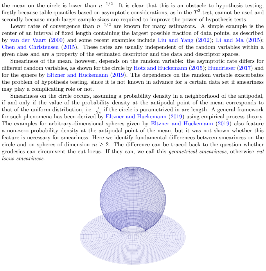
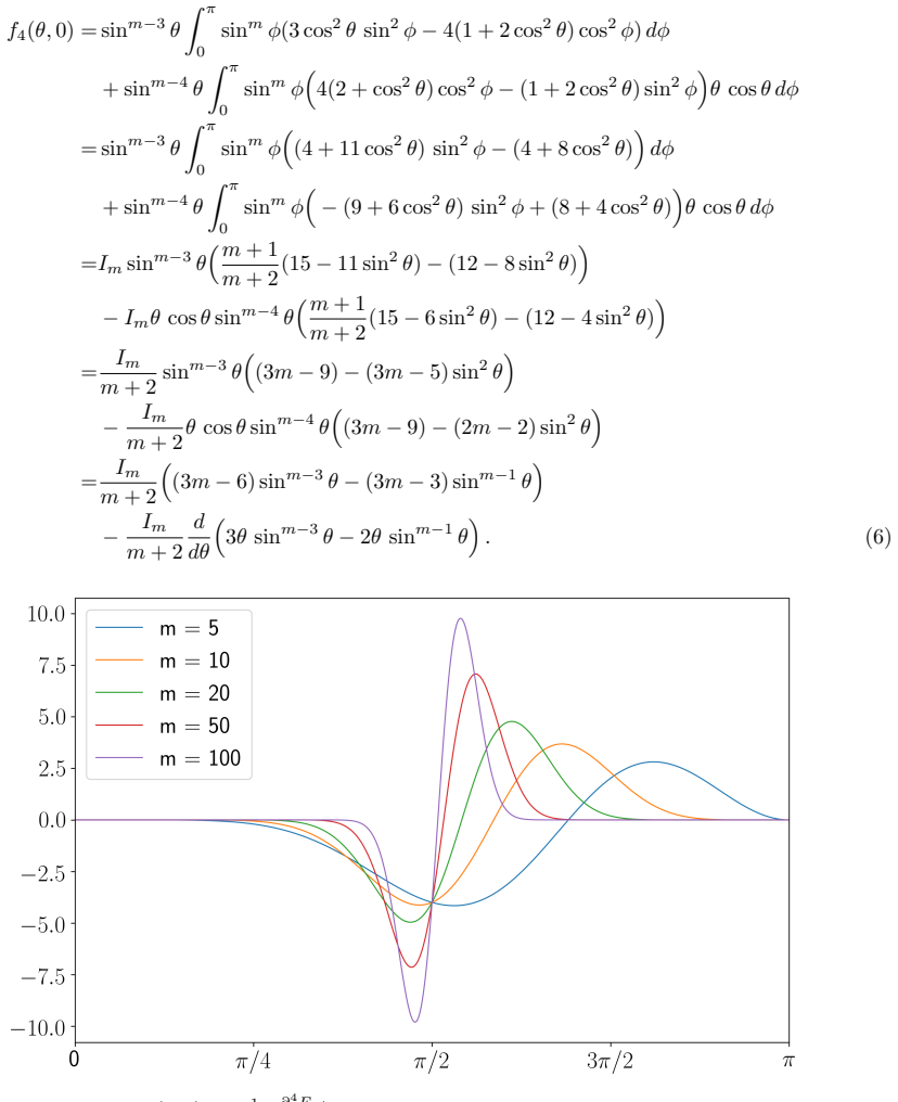
The machinery is the rotationally symmetric Fréchet function $F(\alpha,\beta,\psi)$, where $\psi$ is the polar angle to the north pole $\mu$. Because the measure is invariant under rotations about the polar axis, proving smeariness reduces to showing $\partial^2 F/\partial\psi^2$ vanishes at $\psi=0$ while $\partial^4 F/\partial\psi^4>0$, so the Fréchet function grows like $\psi^4$ and the sample mean fluctuates at $n^{-1/6}$. The spherical annulus $L_{m,\beta}$ is the key object: its hole around the south pole removes the cut locus from the support, isolating the curvature contribution. Geometrical smeariness is smeariness in which the negative Hessian contribution from the cut locus is absent: either $F=G$ in a neighborhood of the mean or $\mathrm{Hess}(F-G)(0)\ge 0$. The proof that the local minimum is global uses Lipschitz bounds (Lemma A.8) on how the second, third, and fourth derivatives of $F$ change with $\beta$, yielding the threshold $\beta_0 = \min(c_m/(2L_4), (1/L_2)\,\partial^2 F/\partial\psi^2(\alpha_0,0,\pi/3))$.
What would settle it
For $m=5$, numerically evaluate the exact Fréchet function $F(\alpha_\beta,\beta,\psi)$ for the uniform annulus plus point mass at the north pole, choosing $\alpha_\beta$ so the Hessian vanishes at $\psi=0$, and check whether $\partial^2 F/\partial\psi^2 > 0$ for all $\psi\in(0,\pi]$ when $\beta\le\beta_0$. If the maximal allowed hole radius is not strictly positive, or if simulations of the sample mean do not show variance scaling like $n^{-1/3}$, the uniqueness-and-rate claim of Theorem 3.1 would be refuted.
Extended reading notes
Core claim
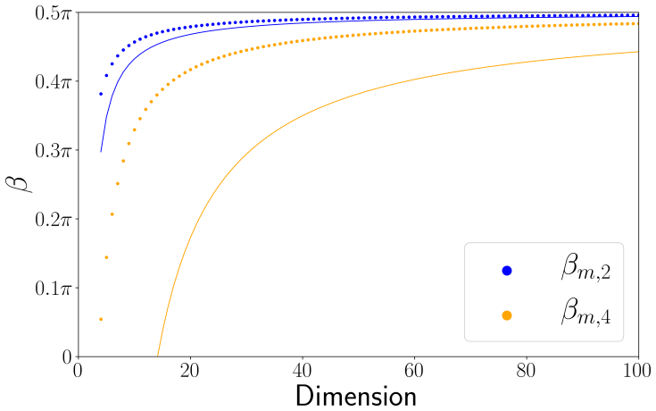
On its own terms, the paper's central discovery is that smeariness on spheres is geometrical, not cut-locus. Theorem 2.10 states that the circle $S^1$ only admits cut locus smeariness, while every sphere $S^m$ with $m\ge 2$ only admits geometrical smeariness: near the mean, the Fréchet function using only geodesics that avoid the cut locus coincides with the full Fréchet function, because geodesics can circumvent the antipodal point. Theorem 3.1 then constructs, for $m\ge 5$, a random variable with a unique 2-smeary Fréchet mean at the north pole whose support excludes a neighborhood of the antipodal point: uniform mass $\alpha$ on the spherical annulus $L_{m,\beta} = \{q : \arccos\langle q,\mu\rangle\in[\pi/2,\pi-\beta]\}$ plus point mass $1-\alpha$ at $\mu$, with $\alpha$ tuned so the Hessian of the Fréchet function vanishes at $\mu$ while its fourth derivative is positive. The resulting asymptotic rate is $n^{-1/6}$, and a corollary deforms the opposite hemisphere to build the same phenomenon on a manifold diffeomorphic to $\mathbb{R}^m$. A further theorem gives a curse of dimensionality: as $m$ grows, the hole radius may approach $\pi/2$, so in high dimension even support barely exceeding a hemisphere can produce smeary local means.
Load-bearing premise
The proof that the local smeary minimum is the unique global mean rests on Lipschitz bounds that are asserted to exist but never explicitly evaluated, and it also assumes the smeary CLT conditions apply to a distribution with a point mass and a hole.
Editorial extensions
If this is right
- On $S^m$ with $m\ge 5$, smeariness can occur even when the support of the random variable has a hole around the cut locus, so the antipodal density is irrelevant.
- A Fréchet mean with vanishing Hessian and positive quartic term has $n^{-1/6}$ fluctuations; the paper shows such means exist concretely on spheres and on manifolds diffeomorphic to $\mathbb{R}^m$.
- Deforming the opposite hemisphere to a flat space yields smeary means on a manifold diffeomorphic to $\mathbb{R}^m$, so topological triviality does not prevent the phenomenon.
- In high dimension, the allowed hole radius grows toward $\pi/2$: random variables whose support barely exceeds a hemisphere can already have smeary local means.
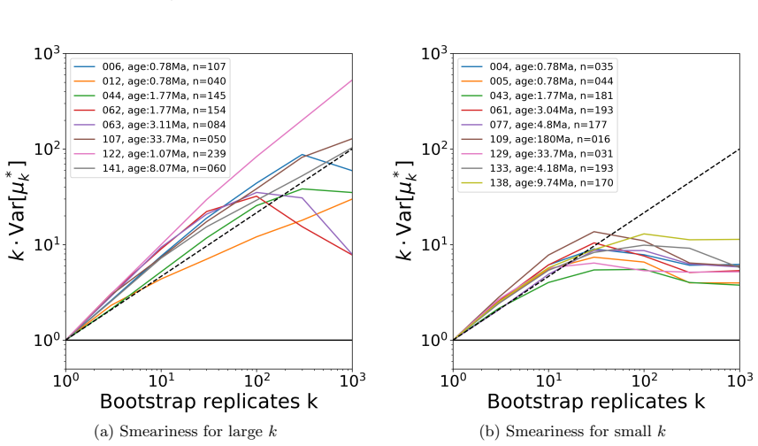
- Finite-sample smeariness of large magnitude is possible for moderately spread spherical data, and the bootstrap analysis of geomagnetic pole-reversal data finds 17 of 151 data sets consistent with it.
Reading between the lines
- Because the Lipschitz constants in the proof are not evaluated, the practical size of the hole radius $\beta_0$ in concrete dimensions is unknown; computing them numerically would show whether the $n^{-1/6}$ regime is robust or confined to a tiny parameter window.
- The same vanishing-Hessian plus positive-quartic mechanism should produce geometrically smeary means on other positively curved, rotationally symmetric spaces, beyond the spheres treated here.
- For practitioners, checking the curvature of the empirical Fréchet function at the estimated mean may be a more useful diagnostic for smeariness than inspecting the density near the antipodal point.
Signed reviews
Editorial analysis
A structured set of objections, weighed in public.
Referee Report
Summary. The paper introduces a distinction between cut-locus smeariness and geometrical smeariness for Fréchet means on Riemannian manifolds. It claims that on the circle smeariness is cut-locus type, while on spheres S^m with m≥2 it is geometrical (Theorem 2.10). The main construction (Theorem 3.1) considers a random variable on S^m, m≥5, uniformly distributed on a spherical annulus L_{m,β} with total mass α plus a point mass at the north pole, and claims that for sufficiently small hole radius β the north pole is the unique Fréchet mean and is 2-smeary with asymptotic rate n^{-1/6}. The paper also proves a curse-of-dimensionality result for the admissible hole radius (Theorem 3.3), discusses finite sample smeariness, presents simulations on Kendall pre-shape space, and analyzes geomagnetic pole reversal data.
Significance. The geometrical-smeariness concept is original and, if established, would be an important contribution to non-Euclidean statistics: it shows that slow n^{-1/6} convergence can occur without probability mass near the cut locus and even on manifolds diffeomorphic to R^m. The supplement contains careful, largely self-contained integral computations for the second and fourth derivatives of the Fréchet function, and the paper is honest about the places where numerical bounds or conjectures are used. The simulations and the geomagnetic data analysis provide a useful practical illustration. At present, however, the formal definition of smeariness is not adequate as written, and the n^{-1/6} claim in Theorem 3.1 is not actually derived; these issues require substantial revision rather than minor polishing.
major comments (4)
- [Definition 2.8] The definition of smeariness only imposes a lower bound: sup_{||x||<δ} |F(x)-F(0)| ≥ C_X δ^κ with κ>2. This condition is automatically satisfied by every Fréchet mean with positive-definite Hessian, because such an F satisfies F(x)-F(0) ≥ c||x||² in a neighborhood, so the supremum over a δ-ball is at least cδ², and for small δ<1 one has cδ² ≥ Cδ^κ for a suitable choice of C. Thus every nondegenerate mean would be classified as smeary, and the definition does not isolate the intended slower-than-n^{-1/2} phenomenon. The definition needs a two-sided growth condition, or an explicit requirement that all derivatives below order κ vanish at 0, to be mathematically meaningful.
- [Theorem 3.1, statement] Theorem 3.1 quantifies over arbitrary total mass 0<α<1 of the uniform annulus component, but the proof uses only the special value α=α_β defined by the condition ∂²F/∂ψ²(α_β,β,0)=0. For generic α the Hessian at the north pole need not vanish, and the claimed n^{-1/6} rate cannot hold; indeed for α<α_β one would expect standard n^{-1/2} asymptotics. The theorem should be restated with α=α_β, or it should be made explicit that the assertion applies only to the tuned value of α.
- [Theorem 3.1, proof / Definition 2.8 note] The asymptotic rate n^{-1/6} is asserted but never derived. Definition 2.8 concerns the population Fréchet function; the distribution of the sample Fréchet mean requires a smeary central limit theorem. The paper's own note after Definition 2.8 says that the smeary asymptotic theory relies on the stricter (Eltzner and Huckemann, 2019, Assumption 2.6), but Theorem 3.1 does not verify that assumption for a distribution with an atom at the mean and an indicator-supported annulus with a hole. In fact, Assumption 2.5(ii) requires a density in a neighborhood of Cut(μ), and the support L_{m,β} with β>0 explicitly excludes such a neighborhood. The theorem should either prove the needed CLT for this case or weaken the claim to '2-smeary in the sense of Definition 2.8' without the n^{-1/6} conclusion.
- [Supplement A.2.1 / Theorem 2.12] Theorem 2.12 states that for every ρ≥0 one can construct a random variable with density value ρ at the south pole and a non-smeary mean at the north pole. The proof, however, sets α=sinδ/(4π) and shows only that the south-pole density can be made arbitrarily large as δ→0. This establishes arbitrarily large density values, not that every nonnegative ρ is attained. A continuity or monotonicity argument over the full range of δ, or a modified construction covering small ρ, is needed; otherwise the theorem should be weakened to 'arbitrarily large ρ'.
minor comments (5)
- [Section 3, proof of Theorem 3.1] The sentence 'This is established by Lemmas A.3 and A.5 in the supplement' appears to cite the wrong lemmas; the local-minimum calculation for the annulus model with a hole is carried out in Lemmas A.6 and A.7.
- [Theorem 3.1 / Definition 2.8] The term '2-smeary' is used in Theorem 3.1 without being defined. Please define k-smeary, or explain the relation between the order κ in Definition 2.8 and the label '2-smeary' and the rate n^{-1/6}.
- [Supplement A.2] The heading 'A.2.1 Proof of Theorem 2.14' should refer to Theorem 2.12, not Theorem 2.14.
- [Supplement A.2.1] The sentence beginning 'No note that due to convexity...' appears to contain a typo ('No note' should likely be 'Note').
- [Lemma A.8 / Eq. (1)] The Lipschitz constants L2, L3, L4 in Lemma A.8 are asserted to exist but are not explicitly bounded, and the threshold β0 in the proof of Theorem 3.1 depends on them. Since the proof argues finiteness, this is not fatal, but an explicit bound or a more transparent finiteness argument would make the uniqueness window quantitative.
Circularity Check
No circularity: Theorem 3.1 is an existence construction with a free parameter tuned to the degeneracy point, and the cited prior work is independent; the unresolved n^{-1/6} issue is a proof gap, not a circular reduction.
full rationale
The central construction is not a fit or a restatement of its inputs. In Theorem 3.1 the free mass parameter αβ is defined by requiring the Hessian to vanish, ∂²F/∂ψ²(αβ,β,0)=0, and the proof then checks by direct integration that the fourth derivative is positive and uses Lipschitz bounds (Lemma A.8) to obtain a unique global minimum for small holes. That is a legitimate mathematical construction, not an estimate renamed as a prediction, and the uniqueness argument is self-contained relative to the β=0 hemisphere model. The citations to Eltzner and Huckemann (2019) supply derivative formulas and a general smeary CLT with stated assumptions; these are prior, independently published results, not assumptions that contain the present conclusion, so the self-citation is not circular. The main caveat is that Theorem 3.1 states the n^{-1/6} asymptotic rate while the proof verifies only the Definition 2.8 growth condition and does not explicitly check the stricter Assumption 2.6 of the cited smeary CLT, and the theorem's quantification over arbitrary α is looser than the proof's α=αβ construction. These are correctness or presentation gaps that do not make the derivation circular.
Assumptions & free parameters
free parameters (2)
- alpha_beta =
Implicitly defined by ∂²F/∂ψ²(αβ,β,0)=0; no closed form given
- alpha_landmark_simulation =
Not reported; described only as making the Hessian slightly positive
assumptions (4)
- domain assumption Assumption 2.5: each random variable has unique population Fréchet mean and a density near the cut locus
- domain assumption Rotation symmetry of the random variables reduces the Fréchet function to a function of polar angle ψ only
- domain assumption VGP data sets are modeled as i.i.d. samples from a fixed spherical distribution
- domain assumption Derivative formulas f2, f4, cm and the smeary CLT from Eltzner and Huckemann (2019) are correct and applicable
Cite this review
Pith. "Pith review of Geometrical Smeariness -- A new Phenomenon of Fr\'echet Means." pith.science (2026). https://pith.science/paper/T2GCDKJM
@misc{pith2026190804233,
  author       = {Pith},
  title        = {Pith review of: Geometrical Smeariness -- A new Phenomenon of Fr\'echet Means},
  year         = {2026},
  howpublished = {\url{https://pith.science/paper/T2GCDKJM}},
  note         = {Machine review of arXiv:1908.04233}
}
abstract
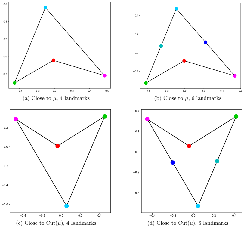
In the past decades, the central limit theorem (CLT) has been generalized to non-Euclidean data spaces. Some years ago, it was found that for some random variables on the circle, the sample Fr\'echet mean fluctuates around the population mean asymptotically at a scale $n^{-\tau}$ with exponent $\tau < 1/2$ with a non-normal distribution if the probability density at the antipodal point of the mean is $\frac{1}{2\pi}$. The author and his collaborator recently discovered that $\tau = 1/6$ for some random variables on higher dimensional spheres. In this article we show that, even more surprisingly, the phenomenon on spheres of higher dimension is qualitatively different from that on the circle, as it depends purely on geometrical properties of the space, namely its curvature, and not on the density at the antipodal point. This gives rise to the new concept of geometrical smeariness. In consequence, the sphere can be deformed, say, by removing a neighborhood of the antipodal point of the mean and gluing a flat space there, with a smooth transition piece. This yields smeariness on a manifold, which is diffeomorphic to Euclidean space. We give an example family of random variables with 2-smeary mean, i.e. with $\tau = 1/6$, whose range has a hole containing the cut locus of the mean. The hole size exhibits a curse of dimensionality as it can increase with dimension, converging to the whole hemisphere opposite a local Fr\'echet mean. We observe smeariness in simulated landmark shapes on Kendall pre-shape space and in real data of geomagnetic north pole positions on the two-dimensional sphere.
Figures

Figures from the paper (6 more)



Reference graph
Works this paper leans on
-
[1]
Afsari, B. (2009). Means and averaging on Riemannian manifolds . University of Maryland
work page 2009
-
[2]
Afsari, B. (2011). Riemannian L ^p center of mass: existence, uniqueness, and convexity. Proceedings of the American Mathematical Society\/ 139 , 655--773
work page 2011
-
[3]
Ahidar-Coutrix, A., T. Le Gouic, and Q. Paris (2019). Convergence rates for empirical barycenters in metric spaces: curvature, convexity and extendable geodesics. Probability Theory and Related Fields\/ 177 , 323--368
work page 2019
-
[4]
Arnaudon, M. and L. Miclo (2014). Means in complete manifolds: uniqueness and approximation. ESAIM: Probability and Statistics\/ 18 , 185--206
work page 2014
- [5]
- [6]
-
[7]
Bhattacharya, A. and R. Bhattacharya (2008). Statistics on riemannian manifolds: asymptotic distribution and curvature. Proceedings of the American Mathematical Society\/ 136 , 2959--2967
work page 2008
-
[8]
Bhattacharya, A. and R. Bhattacharya (2012). Nonparametric Inference on Manifolds . Cambridge University Press
work page 2012
Show all 49 references
-
[9]
Bhattacharya, R. and L. Lin (2017). Omnibus CLT for F r\'echet means and nonparametric inference on non-euclidean spaces. Proceedings of the American Mathematical Society\/ 145\/ (1), 413--428
2017
-
[10]
Bhattacharya, R. N. and V. Patrangenaru (2003). Large sample theory of intrinsic and extrinsic sample means on manifolds I . Annals of Statistics\/ 31\/ (1), 1--29
2003
-
[11]
Bhattacharya, R. N. and V. Patrangenaru (2005). Large sample theory of intrinsic and extrinsic sample means on manifolds II . Annals of Statistics\/ 33\/ (3), 1225--1259
2005
-
[12]
Chen, X. and T. M. Christensen (2015). Optimal Uniform Convergence Rates and Asymptotic Normality for Series Estimators Under Weak Dependence and Weak Conditions . Journal of Econometrics\/ 188\/ (2), 447--465
2015
-
[13]
Clement, B. and D. Kent (1985). A comparison of two sequential geomagnetic polarity transitions (upper olduvai and lower jaramillo) from the southern hemisphere. Physics of the Earth and Planetary Interiors (Special Issue Irregularities in the Secular Variation and Geodynamic ...
1985
-
[14]
Clement, B. and D. Kent (1987). Geomagnetic polarity transition records from five hydraulic piston core sites in the north atlantic. Initial Reports of the Deep Sea Drilling Project\/ 94 , 831--852
1987
-
[15]
Kent, and N
Clement, B., D. Kent, and N. D. Opdyke (1982, 08). Brunhes-matuyama polarity transition in three deep-sea sediment cores. Philosophical Transactions of the Royal Society of London\/ 306 , 113--119
1982
-
[16]
Clement, B. M., L. L. Sierra, E. Smith, and P. Rodda (1996). A record of the upper cochiti polarity transition from the southern hemisphere (fiji). Surveys in Geophysics\/ 17\/ (2), 189--196
1996
-
[17]
Galaz-Garcia, S
Eltzner, B., F. Galaz-Garcia, S. F. Huckemann, and W. Tuschmann (2019). Stability of the cut locus and a central limit theorem for fr \'e chet means of riemannian manifolds. arXiv math.DG 1909.00410\/
2019 arXiv
-
[18]
Eltzner, B. and S. F. Huckemann (2019). A smeary central limit theorem for manifolds with application to high dimensional spheres. Annals of Statistics\/ 47\/ (6), 3360--3381
2019
-
[19]
Groisser, D. (2005). On the convergence of some P rocrustean averaging algorithms. Stochastics: An International Journal of Probability and Stochastic Processes\/ 77\/ (1), 51--60
2005
-
[20]
Gurariy, G. (1988). Geomagnetic field during reversals in the late Cenozoic (Nauka, Moscow) , pp.\ pp. 207. Academy of Sciences of the USSR
1988
-
[21]
Holt, J. W. and J. L. Kirschvink (1995). The upper olduvai geomagnetic field reversal from death valley, california: a fold test of transitional directions. Earth and Planetary Science Letters\/ 133\/ (3), 475--491
1995
-
[22]
Hotz, T. and S. Huckemann (2015). Intrinsic means on the circle: Uniqueness, locus and asymptotics. Annals of the Institute of Statistical Mathematics\/ 67\/ (1), 177--193
2015
-
[23]
Huckemann, H
Hotz, T., S. Huckemann, H. Le, J. S. Marron, J. Mattingly, E. Miller, J. Nolen, M. Owen, V. Patrangenaru, and S. Skwerer (2013). Sticky central limit theorems on open books. Annals of Applied Probability\/ 23\/ (6), 2238--2258
2013
-
[24]
Huckemann, S. (2011a). Inference on 3 D P rocrustes means: Tree boles growth, rank-deficient diffusion tensors and perturbation models. Scandinavian Journal of Statistics\/ 38\/ (3), 424--446
2011
-
[25]
Huckemann, S. (2011b). Intrinsic inference on the mean geodesic of planar shapes and tree discrimination by leaf growth. Annals of Statistics\/ 39\/ (2), 1098--1124
2011
-
[26]
Mattingly, E
Huckemann, S., J. Mattingly, E. Miller, and J. Nolen (2015). Sticky central limit theorems at isolated hyperbolic planar singularities. Electronic Journal of Probability\/ 20\/ (78), 34 pp
2015
-
[27]
Hundrieser, S. (2017). Exploring Smeary Limit Theorems . Bachelor Thesis, University of G\"ottingen
2017
-
[28]
Eltzner, and S
Hundrieser, S., B. Eltzner, and S. Huckemann (2020). Finite sample smeariness of fr\'echet means and application to climate. arXiv stat.ME 2005.02321\/
2020 arXiv
-
[29]
Karcher, H. (1977). Riemannian center of mass and mollifier smoothing. Communications on Pure and Applied Mathematics\/ XXX , 509--541
1977
-
[30]
Karcher, H. (2014). Riemannian center of mass and so called karcher mean. arXiv math.HO 1407.2087\/
2014 arXiv
-
[31]
Nakajima, K
Kawai, N., T. Nakajima, K. Hirooka, and K. Kobayashi (1973). The transition of field at the brunhes and jaramillo boundaries in the matuyama geomagnetic epoch. Proceedings of the Japan Academy\/ 49\/ (10), 820--824
1973
-
[32]
Kendall, W. S. (1990). Probability, convexity, and harmonic maps with small image I : Uniqueness and fine existence. Proceedings of the London Mathematical Society\/ 61 , 371--406
1990
-
[33]
Le, H. (2001). Locating F r\' e chet means with an application to shape spaces. Advances of Applied Probability (SGSA)\/ 33\/ (2), 324--338
2001
-
[34]
Le, H. and D. Barden (2014). On the measure of the cut locus of a F r\'echet mean. Bulletin of the London Mathematical Society\/ 46\/ (4), 698--708
2014
-
[35]
Paris, P
Le Gouic, T., Q. Paris, P. Rigollet, and A. Stromme (2019). Fast convergence of empirical barycenters in alexandrov spaces and the wasserstein space. arXiv math.ST 1908.00828\/
2019 arXiv
-
[36]
Li, Z. and C. Ma (2015). Asymptotic properties of estimators in a stable cox-ingersoll-ross model. Stochastic Processes and their Applications\/ 125\/ (8), 3196--3233
2015
-
[37]
Linssen, J. (1988). Preliminary results of a study of four successive sedimentary geomagnetic reversal records from the mediterranean (upper thvera, lower and upper sidufjall, and lower nunivak). Physics of the Earth and Planetary Interiors\/ 52\/ (3), 207--231
1988
-
[38]
Linssen, J. (1991). Properties of Pliocene sedimentary geomagnetic reversal records from the Mediterranean (Ph.D thesis, University of Utrecht) , Volume 80. Geologica Ultraiectina
1991
-
[39]
Liu, J. and X. Yang (2012). The convergence rate and asymptotic distribution of the bootstrap quantile variance estimator for importance sampling. Advances in Applied Probability\/ 44\/ (3), 815--841
2012
-
[40]
Kent, and J
Mardia, K., J. Kent, and J. Bibby (1979). Mulitvariate Analysis . Probability and Mathematical Statistics. Academic Press
1979
-
[41]
McElhinny, M. W. and J. Lock (1996). IAGA paleomagnetic databases with A ccess. Surveys in Geophysics\/ 17\/ (5), 575--591
1996
-
[42]
Pennec, X. (2019). Curvature effects on the empirical mean in riemannian and affine manifolds: a non-asymptotic high concentration expansion in the small-sample regime. arXiv math.DG 1906.07418\/
2019 arXiv
-
[43]
Rolph, T. C. (1993). The matuyama-jaramillo r-n transition recorded in a loess section near lanzhou, p. r. china. Journal of Geomagnetism and Geoelectricity\/ 45\/ (4), 301--318
1993
-
[44]
Sch\"otz, C. (2019). Convergence rates for the generalized fréchet mean via the quadruple inequality. Electronic Journal of Statistics\/ 13\/ (2), 4280--4345
2019
-
[45]
Sturm, K.-T. (2003). Probability measures on metric spaces of nonpositive curvature. In Heat Kernels and Analysis on Manifolds, Graphs, and Metric Spaces: Lecture Notes from a Quarter Program on Heat Kernels, Random Walks, and Analysis on Manifolds and Graphs , Volume 338, pp....
2003
-
[46]
van der Vaart, A. (2000). Asymptotic Statistics . Cambridge University Press
2000
-
[47]
Van Hoof, A. A. M. and C. G. Langereis (1992). The upper kaena sedimentary geomagnetic reversal record from southern sicily. Journal of Geophysical Research: Solid Earth\/ 97\/ (B5), 6941--6957
1992
-
[48]
van Zijl, J. S. V., K. W. T. Graham, and A. L. Hales (1962). The palaeomagnetism of the stormberg lavas, ii. the behaviour of the magnetic field during a reversal. Geophysical Journal of the Royal Astronomical Society\/ 7\/ (2), 169--182
1962
-
[49]
Wellman, P., M. W. McElhinny, and I. McDougall (1969). On the polar-wander path for australia during the cenozoic. Geophysical Journal International\/ 18\/ (4), 371--395
1969
Reviewed August 14, 2026 · model on record in the stance chip above.
Discussion (0). Continue with ORCID to comment.