REVIEW 2 major objections 5 minor 83 references
The non-homogeneous flow of a thixotropic fluid around a sphere
T0 review · 2 major / 5 minor · reviewed 2026-08-14 · deepseek-v4-flash
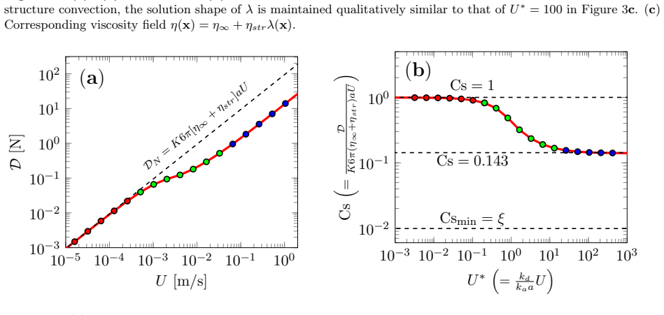
Pith's one-line read A sphere falling through a thixotropic fluid keeps a partially structured wake at high speed, so its drag plateaus near 15 percent of the fully structured value instead of collapsing to the fully broken limit.
desk verdict A clean three-regime picture for thixotropic settling, with one load-bearing caveat: the terminal plateau sits in a regime where the Stokes assumption is no longer obviously valid. read the letter →
The pith
A machine-rendered reading of the paper's core claim, the machinery that carries it, and where it could break.
The reading
What carries the argument
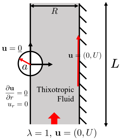
The central object is the structure parameter $\lambda(x)$, whose steady distribution is set by $(u\cdot\nabla)\lambda + k_d\dot{\gamma}_s\lambda - k_a(1-\lambda)=0$, with viscosity $\eta(\lambda)=\eta_\infty+\eta_{\mathrm{str}}\lambda$. The paper solves this coupled advection-reaction structure equation with a discontinuous Galerkin discretization using upwind fluxes inside a Picard iteration around a Stokes solver on an axisymmetric sphere-in-tube domain. Two dimensionless quantities carry the argument: $U^*=(k_d/k_a)U/a$, which compares shear-induced breakdown with Brownian recovery, and $C_s$, the drag normalized by the fully structured Newtonian value including the Faxen wall factor $K$. The convection term in the structure equation is what lets structured fluid arrive from the inlet and prevents $\lambda$ from collapsing to zero at large $U^*$.
What would settle it
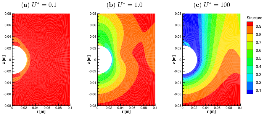
Measure the drag of a calibrated sphere settling in a well-characterized Moore-type thixotropic fluid across $U^*$ from 0.01 to 1000 at fixed confinement; if $C_s$ falls below about 0.10 toward $\xi=0.00990$ at large $U^*$, the convection-balance plateau is falsified. A companion check is to probe the wake structure directly, since the explanation requires a visibly partially structured ($\lambda$ well above zero) wake at $U^*\gg 1$.
Extended reading notes
Core claim
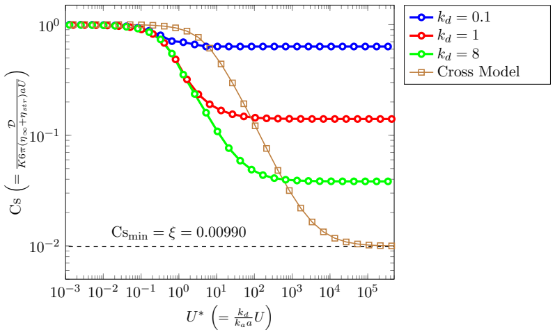
The paper claims that in steady Stokes flow around a settling sphere, a Moore thixotropic fluid cannot reach its fully broken state at high falling speeds. Although steady simple shear would drive the structure parameter $\lambda$ to nearly zero and the viscosity to $\eta_\infty$, the sphere flow does not: convection brings fully structured ($\lambda=1$) fluid from upstream faster than shear can destroy it, so a partially structured region, especially the wake, survives. As a result the drag coefficient $C_s = D/[K\,6\pi(\eta_\infty+\eta_{\mathrm{str}}) a U]$ follows a sigmoid with $U^* = (k_d/k_a)U/a$ and levels off near $C_s\approx 0.15$, roughly fifteen times the fully broken floor $\xi=\eta_\infty/(\eta_\infty+\eta_{\mathrm{str}})=0.00990$. The same balance explains why the flow at $U^*=200$ is fore-aft asymmetric and why pressure drag is about twice the viscous drag, the opposite of the Newtonian creeping-flow partition.
Load-bearing premise
The load-bearing premise is that creeping Stokes flow remains the right momentum balance throughout the $U^*$ sweep; at the fastest speeds the paper estimates local Reynolds numbers up to 0.8, so inertia could alter the plateau.
Editorial extensions
If this is right
- If the plateau is real, drag at high terminal velocities grows linearly with speed but with effective viscosity roughly $0.15(\eta_\infty+\eta_{\mathrm{str}})$, so standard Stokes-calibrated settling estimates would overpredict the resistance and underpredict the settling time.
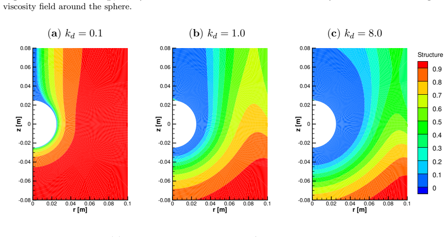
- A finite destruction parameter $k_d$ is what separates thixotropic behavior from a generalized Newtonian Cross fluid in this geometry: at large $U^*$ the Cross fluid falls to $\xi$, while the thixotropic fluid stays on the plateau, and increasing $k_d$ pulls the plateau down toward $\xi$.
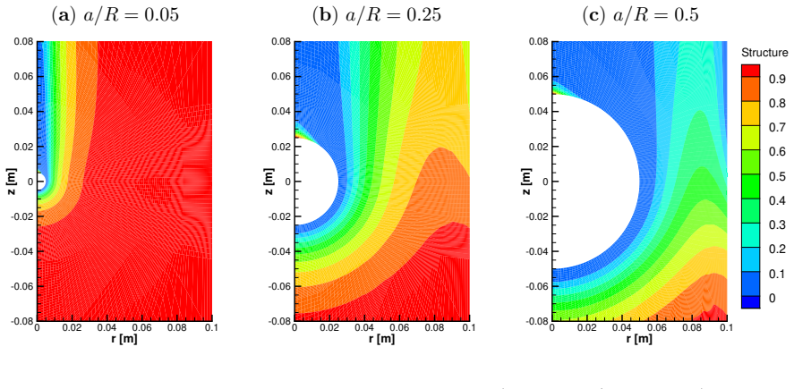
- Confinement changes not only the plateau level but also the shape of the transient regime: a larger $a/R$ makes $C_s$ drop earlier and to a lower floor, so flow geometry can be tuned to control effective thixotropic resistance without changing the material.
- If nonlinearity is added to the viscosity function ($\eta=\eta_\infty+\eta_{\mathrm{str}}\lambda^2$), the plateau moves to about $0.095$ but stays far above $\xi$; if instead a quadratic shear term is added to the kinetics equation, the structure eventually breaks fully and the drag approaches the Newtonian $\eta_\infty$ limit.
- The plateau level itself encodes the balance between breakdown and convection, so it provides a single-number diagnostic for how strongly microstructure is being replenished in any given flow geometry.
Reading between the lines
- Editorial inference: A direct test of the mechanism is to run the same fluid in a closed recirculating geometry, where the upstream fluid has already been sheared; the plateau should shrink or vanish because convection can no longer supply fresh structure from an undisturbed reservoir.
- Editorial inference: The ratio $C_s^{\mathrm{plateau}}/\xi$ could serve as a practical convective-compensation factor for a thixotropic fluid in a chosen geometry, measurable from a settling curve and useful for process design without needing full structure-field measurements.
- Editorial inference: The paper's own Reynolds estimate reaches up to about 0.8 in the fastest cases, so the precise plateau value may shift once inertia is included; repeating the sweep at matched low Reynolds numbers by raising the fluid viscosity would isolate the thixotropic-convection contribution from inertial drag.
- Editorial inference: For non-spherical particles or bubbles the stagnation-point and wake topology changes, so the plateau level should depend on shape; this could make the high-$U^*$ plateau a shape-sensitive fingerprint of thixotropic microstructure.
Signed reviews
Editorial analysis
A structured set of objections, weighed in public.
Referee Report
Summary. The paper presents numerical simulations of steady creeping flow of a Moore-type thixotropic fluid around a settling sphere in a cylindrical tube. The structure-kinetics equation (7) is solved with a discontinuous Galerkin method coupled to Stokes equations (5)-(6) through a viscosity that depends on the structure parameter λ. Based on the normalized velocity U* = t_c U/a, the paper identifies three regimes: a Newtonian-like regime at U* << 1, a transient regime, and a terminal regime at U* >> 1 in which the drag coefficient C_s (defined by Eq. (17)) approaches a plateau near 0.15 rather than the fully-broken limit ξ = 0.00990. The plateau is attributed to a balance between shear-induced structure breakdown and the convection of fully-structured fluid from upstream, in contrast to the homogeneous limit where Brownian recovery alone is balanced. The paper also studies the effects of the destruction parameter k_d, the viscosity ratio ξ, the confinement ratio a/R, and two forms of nonlinear model modifications.
Significance. If the terminal-plateau mechanism is correct, the paper provides a concrete, falsifiable prediction: in non-homogeneous thixotropic flow, the drag coefficient does not approach the fully-broken viscosity ratio ξ as U* grows, because convection of unbroken structure from upstream sustains a finite effective viscosity near the sphere. This is a useful conceptual step beyond homogeneous rheometry for interpreting settling and processing flows. The numerical scheme is verified by a manufactured-solution test showing third-order convergence (Appendix A), and the model parameters (Table 1) are generic, not fitted to the reported drag, so the plateau is a genuine model output rather than a fitted curve. The main limitation is that the central plateau claim is computed under the Stokes assumption in a regime where local Reynolds numbers may not be small, and the paper does not provide a mesh-refinement study for the actual settling problem. These issues are examined in the major comments.
major comments (2)
- [Section 3, Figure 5(b)] The central claim that C_s plateaus near 0.15 for U* >> 1 rests on solutions of the Stokes equations (5)-(6), but the terminal regime is explored in a range where the creeping-flow assumption is questionable. With the paper's own parameters (ρ_f ≈ 1000 kg/m^3, a = 0.025 m, t_c = 10 s), U* = 100 and 1000 correspond to U = 0.25 and 2.5 m/s. In the strongly broken region near the sphere the viscosity approaches η_∞ = 1 Pa·s, giving local Re = ρ_f U a / η ≈ 6 and 62, respectively; even at the lower edge of the claimed plateau, U* = 10 (U = 0.025 m/s), the fully-broken value gives Re ≈ 0.6. The paper's statement that Re is at most 0.8 is based on a viscosity of 100–15 Pa·s, which is not representative of the thin broken layer that controls the drag. If inertia is included, u and γ̇_s no longer scale linearly with U, so the structure balance (7) is no longer independent of U and the plateau in C_s may be an artifact of the Stokes assumption. Please add either (i) inertial (Navier–Stokes) simulations for at least a few high-U* cases to test whether the plateau persists, or (ii) a posteriori Re-field evaluation with a clear statement of the U* range in which Re < 0.1, and restrict the plateau claim accordingly.
- [Section 2.4 and Appendix A] The manufactured-solution test in Appendix A confirms the formal third-order convergence of the discretization, but it does not establish that the reported C_s values—particularly the terminal plateau near 0.15—are mesh-converged on the 49,152-element mesh used for all results. The structure equation is a hyperbolic advection-reaction equation with sharp structure gradients near the sphere (e.g., Fig. 3c), and the drag integral (13) depends sensitively on near-sphere resolution. Please provide a mesh-refinement study for at least two representative conditions (e.g., U* = 0.1 and U* = 100) demonstrating that C_s changes by less than a few percent between the two finest meshes. Without this, the quantitative plateau values reported in Figures 5, 8, 9, 11, and 13 should be treated as tentative.
minor comments (5)
- [Section 3, Figure 5] The terminal value of C_s is reported inconsistently: the text says it converges to 0.15, while the caption of Figure 5(b) states C_s = 0.143, and later figures quote 0.104 and 0.194 without explaining how these constants are extracted. Please harmonize the numbers and state the criterion used to identify the plateau value.
- [Section 3, Figure 5(a)] The x-axis of Figure 5(a) extends only to U = 1 m/s, but the terminal regime at U* = 10^3 corresponds to U = 2.5 m/s with the given a and t_c, so the claimed linear D-U dependence in the terminal regime is not visible in the plot. Please extend the axis or add an inset.
- [Section 2.3] The normalized velocity is defined as U* = t_c U/a in Eq. (15), but figure axes use the equivalent expression U* = (k_d/k_a a) U (e.g., Figure 5b). Please use a single notation throughout and define it once in the text.
- [Abstract and Section 6] The phrase 'thixotropy fluid' in the abstract should be 'thixotropic fluid', and 'Discontinous Galerkin' in Section 6 should be 'Discontinuous Galerkin'.
- [Appendix A] The manufactured solution for λ (Eq. A.4) is unbounded and exceeds the physical range λ ∈ [0,1]; the authors correctly note this is acceptable for code verification, but a bounded manufactured solution would also exercise the physical constraints and the upwind treatment at boundaries more realistically.
Circularity Check
No significant circularity: the terminal plateau in Cs is an emergent simulation output, and the model parameters are not fitted to the reported drag behavior.
full rationale
The paper's central claims—the three flow regimes and the terminal plateau near Cs ≈ 0.15 at U* >> 1—are outputs of the coupled Stokes-flow / structure-kinetics solver, not inputs. The four model parameters in Table 1 (η∞=1 Pa·s, ηstr=100 Pa·s, ka=0.1 s⁻¹, kd=1) are chosen as a generic thixotropic fluid and are not calibrated to any drag measurement; the Cs–U* curve and the plateau value emerge from the simulation. The large-U* plateau is additionally supported by an independent scaling argument based on Eq. (7): after non-dimensionalization, the Brownian recovery term is O(1/U*) and drops out, leaving the U*-independent balance (u·∇λ) + kd γ̇s λ = 0 in Stokes flow. This explains, rather than presupposes, the numerically observed plateau. The two author-overlapping citations (refs 37 and 53) are used only to point to prior numerical procedures and prior use of the Moore model; they provide no fitted parameter, no uniqueness theorem, and no definition of Cs, so they are not load-bearing. The paper’s own acknowledgment that the Reynolds number may reach ≈0.8 at high U* (Sec. 3) is a validity limitation for the Stokes assumption, not a circularity. No derivation reduces to its own input by construction, and no fitted quantity is relabeled as a prediction.
Assumptions & free parameters
free parameters (5)
- eta_infinity (residual viscosity) =
1.0 Pa.s
- eta_str (structural viscosity) =
100.0 Pa.s
- ka (Brownian recovery rate) =
0.1 s^-1
- kd (destruction parameter) =
1.0 (dimensionless)
- kd2 (nonlinear kinetic coefficient) =
1.0 s
assumptions (5)
- domain assumption Stokes flow (Re << 1) applies for all simulated U*
- domain assumption Steady state (d/dt = 0) is reached
- domain assumption Axisymmetric flow in a cylindrical tube
- domain assumption Fully structured fluid enters at the upstream boundary (lambda = 1)
- domain assumption Linear Moore model captures generic thixotropy
Cite this review
Pith. "Pith review of The non-homogeneous flow of a thixotropic fluid around a sphere." pith.science (2026). https://pith.science/paper/T4T4ANNR
@misc{pith2026190804993,
  author       = {Pith},
  title        = {Pith review of: The non-homogeneous flow of a thixotropic fluid around a sphere},
  year         = {2026},
  howpublished = {\url{https://pith.science/paper/T4T4ANNR}},
  note         = {Machine review of arXiv:1908.04993}
}
abstract
The non-homogeneous flow of a thixotropic fluid around a settling sphere is simulated. A four-parameter Moore model is used for a generic thixotropic fluid and discontinuous Galerkin method is employed to solve the structure-kinetics equation coupled with the conservation equations of mass and momentum. Depending on the normalized falling velocity $U^{*}$, which compares the time scale of structure formation and destruction, flow solutions are divided into three different regimes, which are attributed to an interplay of three competing factors: Brownian structure recovery, shear-induced structure breakdown, and the convection of microstructures. At small $U^{*}( \ll 1)$, where the Brownian structure recovery is predominant, the thixotropic effect is negligible and flow solutions are not too dissimilar to that of a Newtonian fluid. As $U^{*}$ increases, a remarkable structural gradient is observed and the structure profile around the settling sphere is determined by the balance of all three competing factors. For large enough $U^{*}(\gg 1)$, where the Brownian structure recovery becomes negligible, the balance between shear-induced structure breakdown and the convection plays a decisive role in determining flow profile. To quantify the interplay of three factors, the drag coefficient Cs of the sphere is investigated for ranges of $U^{*}$. With this framework, the effect of the destruction parameter, the confinement ratio, and a possible nonlinearity in the model-form on the non-homogeneous flow of a thixotropy fluid have been addressed.
Figures

Figures from the paper (11 more)





Reference graph
Works this paper leans on
-
[1]
Mewis and N
J. Mewis and N. J. Wagner. Colloidal Suspension Rheology, chapter Thixotropy, pages 228–251. Cambridge Series in Chemical Engineering. Cambridge University Press, 2011
2011
-
[2]
R. G. Larson and Y. Wei. A review of thixotropy and its rheological modeling. Journal of Rheology, 63:477–501, 2019
2019
-
[3]
Dullaert and J
K. Dullaert and J. Mewis. A structural kinetics model for thixotropy. Journal of Non-Newtonian Fluid Mechanics, 139:21–30, 2006
2006
-
[4]
J. Engmann and A. S. Burbidge. Fluid mechanics of eating, swallowing and digestion - overview and perspectives. Food & Function, 4:443–447, 2013
work page 2013
-
[5]
D. Quemada and R. Droz. Blood viscoelasticity and thixotropy from stress formation and relaxation measurements: a unified model. Biorheology, 20:635–651, 1983
work page 1983
-
[6]
R. G. de Krester and D. V. Boger. A structural model for the time-dependent recovery of mineral suspensions. Rheologica Acta, 40:582–590, 2001
work page 2001
-
[7]
Peptide-Based Physical Gels Endowed with Thixotropic Behaviour. N. zanna and c. tomasini. Gels, 3:39, 2017
work page 2017
-
[8]
S. Mortazavi-Manesh and J. M. Shaw. Thixotropic rheological behavior of maya crude oil. Energy & Fuels, 28:972–979, 2014
work page 2014
Show all 83 references
-
[9]
Armelin, M
E. Armelin, M. Mart´ ı, E. Rud´ e, J. Labanda, J. Llorens, and C. Alem´ an. A simple model to describe the thixotropic behavior of paints. Progress in Organic Coatings, 57(3):229–235, 2006
2006
-
[10]
H. A. Barnes. Thixotropy—a review. Journal of Non-Newtonian Fluid Mechanics , 70(1–2):1–33, 1997
1997
-
[11]
Mewis and N
J. Mewis and N. J. Wagner. Thixotropy. Advances in Colloid and Interface Science , 147– 148:214–227, 2009
2009
-
[12]
C. F. Goodeve. A general theory of thixotropy and viscosity. Transactions of Faraday Society, 35:342–358, 1939
1939
-
[13]
F. Moore. The rheology of ceramic slips and bodies. Transactions and journal of British Ceramic Society, 58:470–494, 1959
1959
-
[14]
Stickel, R
J. Stickel, R. J. Phillips, and R. L Powell. A constitutive model for microstructure and total stress in particulate suspensions. Journal of Rheology, 50:379, 2006
2006
-
[15]
J. D. Goddard. Dissipative materials as models of thixotropy and plasticity. Journal of Non-Newtonian Fluid Mechanics , 14:141–160, 1984
1984
-
[16]
P. D. Patel and W. B. Russel. A mean field theory for the rheology of phase separated or flocculated dispersions. Colloids and Surfaces , 31:355–383, 1988
1988
-
[17]
A. A. Potanin. On the mechanism of aggregation in the shear flow of suspensions. Journal of Colloid and Interface Science , 145:140–157, 1991. 24
1991
-
[18]
D. S. Dickey and J. B. Fasano. How geometry and viscosity influence mixing. Chemical Engineering, 111:42–46, 2004
2004
-
[19]
A. B. Metzner and R. E. Otto. Agitation of nonNewtonian fluids. AIChE Journal, 3:3–10, 1957
1957
-
[20]
J. E. L´ opez-Aguilar, M. F. Webster, H. R. Tamaddon-Jahromi, and O. Manero. A comparative numerical study of time-dependent structured fluids in complex flows. Rheologica Acta, 55:197– 214, 2016
2016
-
[21]
J. E. L´ opez-Aguilar, M. F. Webster, H. R. Tamaddon-Jahromi, and O. Manero. Numerical modelling of thixotropic and viscoelastoplastic materials in complex flows. Rheologica Acta, 54:307–325, 2014
2014
-
[22]
J. E. L´ opez-Aguilar, M. F. Webster, H. R. Tamaddon-Jahromi, and O. Manero. High-weissenberg predictions for micellar fluids in contraction–expansion flows. Journal of Non-Newtonian Fluid Mechanics, 222:190–208, 2015
2015
-
[23]
J. E. L´ opez-Aguilar, M. F. Webster, H. R. Tamaddon-Jahromi, and O. Manero. A new constitutive model for worm-like micellar systems – numerical simulation of confined contraction– expansion flows. Journal of Non-Newtonian Fluid Mechanics , 204:7–21, 2014
2014
-
[24]
P. Coussot. Yield stress fluid flows: A review of experimental data. Journal of Non-Newtonian Fluid Mechanics, 211:31–49, 2014
2014
-
[25]
A. N. Beris, J. A. Tsamopoulos, R. C. Armstrong, and R.A. Brown. Creeping motion of a sphere through a Bingham plastic. Journal of Fluid Mechanics , 1588:219–244, 1985
1985
-
[26]
Blackery and E
J. Blackery and E. Mitsoulis. Creeping motion of a sphere in tubes filled with a Bingham plastic material. Journal of Non-Newtonian Fluid Mechanics , 70:59–77, 1997
1997
-
[27]
Tripathi and R
A. Tripathi and R. P. Chhabra. Drag on spheroidal particles in dilatant fluids. AIChE Journal, 41:728–731, 1995
1995
-
[28]
S. Tian. Wall effect for spherical partical in confined shear-thickening fluids. Journal of Non-Newtonian Fluid Mechanics , 257:13–21, 2018
2018
-
[29]
Gervang, A
B. Gervang, A. R. Davies, and T. N. Phillips. On the simulation of viscoelastic flow past a sphere using spectral methods. Journal of Non-Newtonian Fluid Mechanics , 44:281–306, 1992
1992
-
[30]
P. Y. Huang and J. Feng. Wall effects on the flow of viscoelastic fluids around a circular cylinder. Journal of Non-Newtonian Fluid Mechanics , 60:179–198, 1995
1995
-
[31]
Ferroir, H
T. Ferroir, H. Huynh, and X. Chateau P. Coussot. Motion of a solid object through a pasty (thixotropic) fluid. Physics of Fluids , 16(3):594–601, 2004
2004
-
[32]
Maleki-Jirsaraei, S
N. Maleki-Jirsaraei, S. Hassani, and S. Azizi. Settling of spherical objects through thixotropic fluids: A statistical approach. Modern Applied Science, 12:72–76, 2018
2018
-
[33]
M. M. Gumulya, R. R. Horsley, and V. Pareek. Numerical simulations of the settling behavior of particles in thixotropic fluids. Physics of Fluids , 26, 2014. 25
2014
-
[34]
M. M. M. Thant, M. T. M. Sallehud-Din, G. Hewitt, C. Hale, and J. Quarini. Mitigating flow assurance challenges in deepwater fields using active heating methods. Society of Petroleum Engineer, 2011
2011
-
[35]
C. R. Huang and W. Fabisiak. Thixotropic parameters of whole human blood. Thrombosis Research,, 8:1–8, 1976
1976
-
[36]
J. J. Derksen. Simulations of thixotropic liquids. Applied Mathematical Modeling, 35(4):1656– 1665, 2011
2011
-
[37]
J. B. Freund, J. Kim, and R. H. Ewoldt. Field sensitivity of flow predictions to rheological parameters. Journal of Non-Newtonian Fluid Mechanics , 257, 2018
2018
-
[38]
C. M. Rodkiewicz, editor. Arteries and Arterial Blood Flow: Biological and physiological aspects . CISM International Centre for Mechanical Sciences. Springer-Verlag Wien, 1st edition, 1983
1983
-
[39]
A. Tehrani. Thixotropy in water-based drilling fluids. Annual Transactions of the nordic rheology society, 16:1–13, 2008
2008
-
[40]
Happel and H
J. Happel and H. Brenner. Low Reynolds number hydrodynamics. Prentice-Hall, London, 1965
1965
-
[41]
Tabuteau, P
H. Tabuteau, P. Coussot, and J. de Bruyn. Drag force on a sphere in steady motion through a yield-stress fluid. Journal of Rheology, 51(1):125–137, 2007
2007
-
[42]
Arndt, W
D. Arndt, W. Bangerth, D. Davydov, T. Heister, L. Heltai, M. Kronbichler, M. Maier, J. P. Pelteret, B. Turcksin, and D. Wells. The deal.II library, version 8.5. Journal of Numerical Mathematics, 2017
2017
-
[43]
Bangerth, R
W. Bangerth, R. Hartmann, and G. Kanschat. deal.II — a general purpose object oriented finite element library. ACM Trans. Math. Softw. , 33(4):24/1–24/7, 2007
2007
-
[44]
Taylor and P
C. Taylor and P. Hood. A numerical solution of the navier-stokes equations using the finite element technique. Computers & Fluids , 1:73–100, 1973
1973
-
[45]
J. S. Hesthaven and T. Warburton. Nodal Discontinuous Galerkin Methods: Algorithms, Analysis, and applications. Texts in Applied Mathematics. Springer-Verlag New York, 2008
2008
-
[46]
Saramito
P. Saramito. Complex Fluids: Modeling and Algorithms , volume 79 of Math´ ematiques et Applications. Springer, 2016
2016
-
[47]
Saad and M
Y. Saad and M. H. Schultz. GMRES: A generalized minimal residual algorithm for solving nonsymmetric linear systems. SIAM Journal on Scientific Computing , 7:856–869, 1986
1986
-
[48]
R. C. Mittal and. A. H. AL-Kurdi. An efficient method for constructing an ilu preconditioner for solving large sparse nonsymmetric linear systems by the gmres method. Computers & Mathematics with applications , 45:1757–1772, 2003
2003
-
[49]
R. B. Bird, R. C. Armstrong, and O. Hassager. Dynamics of Polymeric Liquids, Vol. 1: Fluid mechanics. Wiley, 2nd edition, 1987
1987
-
[50]
Fraggedakis, Y
D. Fraggedakis, Y. Dimakopoulos, and J. Tsamopoulos. Yielding the yield-stress analysis: a study focused on the effects of elasticity on the settling of a single spherical particle in simple yield-stress fluids. Soft Matter, 12(24):5378–5401, 2016. 26
2016
-
[51]
M. M. Cross. Rheology of non-newtonian fluids: A new flow equation for pseudoplastic systems. Journal of Colloid Science , 20:417–437, 1965
1965
-
[52]
panta rei
Howard A. Barnes. The yield stress—a review or “panta rei ”— everything flows? Journal of Non-Newtonian Fluid Mechanics , 81(1):133 – 178, 1999
1999
-
[53]
J. Kim, P. K. Singh, J. B. Freund, and R. H. Ewoldt. Uncertainty propagation in simulation predictions of generalized newtonian fluid flows. Journal of Non-Newtonian Fluid Mechanics , 271:104138, 2019
2019
-
[54]
Mitsoulis and J
E. Mitsoulis and J. Tsamopoulos. Numerical simulations of complex yield-stress fluid flows. Rheologica Acta, 56:231–258, 2017
2017
-
[55]
N. J. Balmforth, I. A. Frigaard, and G. Ovarlez. Yielding to stress: Recent developments in viscoplastic fluid mechanics. Annual Review of Fluid Mechanics , 46:121–146, 2014
2014
-
[56]
H. A. Ardakani, E. Mitsoulis, and S. G. Hatzikiriakos. Thixotropic flow of toothpaste through extrusion dies. Journal of Non-Newtonian Fluid Mechanics , 166:1262–1271, 2011
2011
-
[57]
A. N. Alexandrou, N. Constantinou, and G. Georgiou. Shear rejuvenation, aging and shear banding in yield stress fluids. Journal of Non-Newtonian Fluid Mechanics , 158:6–17, 2009
2009
-
[58]
R. L. Thompson, L. U. R. Sica, and P. R. S. Mendes. The yield stress tensor. Journal of Non-Newtonian Fluid Mechanics , 261:211–219, 2018
2018
-
[59]
everything flows?
M. Dinkgreve, M. M. Denn, and D. Bonn. “everything flows?”: elastic effects on startup flows of yield-stress fluids. Rheologica Acta, 56(3):189–194, 2017
2017
-
[60]
J. E. L´ opez-Aguilar, M. F. Webster, H. R. Tamaddon-Jahromi, and O. Manero. Predictions for circular contraction-expansion flows with viscoelastoplastic & thixotropic fluids. Journal of Non-Newtonian Fluid Mechanics , 261:188–210, 2018
2018
-
[61]
Renardy and Y
M. Renardy and Y. Renardy. Thixotropy in yield stress fluids as a limit of viscoelasticity. IMA Journal of Applied Mathematics , 3:522–537, 2016
2016
-
[62]
S Stephanou and G
P. S Stephanou and G. G. Georgiou. A nonequilibrium thermodynamics perspective of thixotropy. The Journal of Chemical Physics , 149:244902, 2018
2018
-
[63]
S. F. Lin and R. S. Brodkey. Rheological properties of slurry fuels. Journal of Rheology , 29(2):147–175, 1985
1985
-
[64]
K. L. Pinder. Time dependent rheology of the tetrahydrofuran-hydrogen sulphide gas hydrate slurry. The Canadian Journal of Chemical Engineering , 42:132–138, 1964
1964
-
[65]
G. R. Burgos, A. N. Alexandrou, and V. Entov. Thixotropic rheology of semisolid metal suspensions. Journal of Materials Processing Technology, 110:164–176, 2001
2001
-
[66]
J. B. Freund and R. H. Ewoldt. Quantitative rheological model selection: Good fits versus credible models using Bayesian inference. Journal of Rheology, 59:667–701, 2015
2015
-
[67]
H. Jeffreys. Theory of Probability. Oxford University Press, 3rd edition, 1961
1961
-
[68]
X. Yang, H. Huang, and X. Lu. Sedimentation of an oblate ellipsoid in narrow tubes. Physical Review E, 92:063009, 2015. 27
2015
-
[69]
I. E. Kareva and V. L. Sennitskii. Motion of a circular cylinder in a vibrating liquid. Journal of Applied Mechanics and Technical Physics , 42:276–278, 2001
2001
-
[70]
Agarwal and R
N. Agarwal and R. P. Chhabra. Settling velocity of cubes in newtonian and power law liquids. Powder Technology, 178:17–21, 2007
2007
-
[71]
Sarpkaya
T. Sarpkaya. Forces on cylinders and spheres in a sinusoidally oscillating fluid. Journal of Applied Mechanics, 42:32–37, 1974
1974
-
[72]
V. L. Sennitskii. Motion of a sphere in a vibrating liquid in the presence of a wall. Journal of Applied Mechanics and Technical Physics , 40:662–668, 1999
1999
-
[73]
Zhang, C
L. Zhang, C. Yang, and Z-S. Mao. Numerical simulation of a bubble rising in shear-thinning fluids. Journal of Non-Newtonian Fluid Mechanics , 165:555–567, 2010
2010
-
[74]
W. C. Chin. Computational Rheology for Pipeline and Annular Flow: Non-Newtonian Flow Modeling for Drilling and Production, and Flow Assurance Methods in Subsea Pipeline Design . Elsevier Science, 2001
2001
-
[75]
Ratulowski A
Ahmed J. Ratulowski A. Hammami. Precipitation and Deposition of Asphaltenes in Production Systems: A Flow Assurance Overview , pages 617–660. Springer New York, New York, NY, 2007
2007
-
[76]
Bonn and M
D. Bonn and M. M. Denn. Yield stress fluid slowly yield to analysis. Science, 324:1401–1402, 2009
2009
-
[77]
M. M. Denn and D. Bonn. Issues in the flow of yield-stress liquids. Rheologica Acta, 50(4):307– 315, 2011
2011
-
[78]
P. R. S. Mendes. Thixotropic elasto-viscoplastic model for structured fluids. Soft Matter , 7(6):2471–2483, 2011
2011
-
[79]
C. J. Roy. Review of code and solution verification procedures for computational simulation. Journal of Computational Physics , 205:131–156, 2005
2005
-
[80]
Steinberg and P
S. Steinberg and P. J. Roache. Symbolic manipulation and computational fluid dynamics. Journal of Computational Physics , 57:251–284, 1985
1985
-
[81]
P. J. Roache. Code verification by the Method of Manufactured solutions. Journal of Fluids Engineering, 124:4–10, 2001
2001
-
[82]
Babuska and S
I. Babuska and S. Szabo. On the rates of convergence of the finite element method. International Journal for Numerical Method for Engineering , 18:323–341, 1982
1982
-
[83]
Brenner and L
S. Brenner and L. R. Scott. The mathematical theory of finite element method , volume 15 of Texts in Applied Mathematics . Springer-Verlag New York, 2002. 28
2002
Reviewed August 14, 2026 · model on record in the stance chip above.
Discussion (0). Continue with ORCID to comment.