Residual-Based Time Discretization on Nonlinear Approximation Manifolds: Analysis and Gaussian Applications

Caroline Lasser; Eddy de Leon

REVIEW 3 major objections 4 minor 29 references

Residual-Based Time Discretization on Nonlinear Approximation Manifolds: Analysis and Gaussian Applications

T0 review · 3 major / 4 minor · reviewed 2026-08-02 · deepseek-v4-flash

Challenge this review Re-run · record.json Download PDF Read on arXiv ↗

Pith's one-line read This paper proves that two residual-based time-stepping schemes on nonlinear approximation manifolds — discretize-then-parametrize and parametrize-then-discretize — obey error bounds that separate the residual-minimization error from the ti

desk verdict A genuinely useful unified error analysis for residual-based time stepping, but the parametrize-then theorem's hypotheses fail on the paper's own Gaussian manifolds, so the application needs revision. read the letter →

arxiv 2607.15086 v1 pith:TDRH765H submitted 2026-07-16 math.NA cs.NAquant-ph

Eddy de Leon , Caroline Lasser This is my paper · ORCID

classification math.NAcs.NAquant-ph MSC 65M1265M1565L2041A3065D15

keywords residual-basedtimesteppingnonlinearmanifoldapproximationζ-methodsDirac–FrenkelvariationalprincipleGaussianconvergenceanalysisevolutionequationsinHilbertspacesSchrödingerdynamics

verification ladder T0 review T1 audit T2 compute T3 formal

The pith

A machine-rendered reading of the paper's core claim, the machinery that carries it, and where it could break.

The reading

This paper gives a single error analysis for two ways of stepping approximate solutions of evolution equations along a nonlinear manifold. In the discretize-then-parametrize approach, a ζ-method (Euler or trapezoidal-type) is applied to the equation first, then each new state is chosen by minimizing the residual in the Hilbert space norm. In the parametrize-then-discretize approach, the Dirac–Frenkel tangent-space projection is discretized instead. The main result is that the global error is bounded by the initialization error plus two additive terms: a residual-minimization contribution ρ/h and a classical time-discretization term c_s h^s, with s=1 for general ζ and s=2 for the midpoint choice. The parametrize-then variant carries an extra constant that depends on the smallest singular value of the averaged parameter gradient, quantifying the penalty for near-tangent-space collapse. The paper also derives closed-form Gaussian integrals that make the residual and its gradient computable without a spatial grid when the evolution operator acts polynomially.

What carries the argument

The ζ-method residual family: for a parameter θ_k, the discretize-then residual is u(θ,·)−u(θ_k,·)−h[ζ f(t_k,u(θ_k))+ζ̂ f(t,u(θ))], and the parametrize-then residual replaces the difference u(θ,·)−u(θ_k,·) by the linearized increment [ζ∇θu(θ_k)+ζ̂∇θu(θ)](θ−θ_k). The cost function F_k(θ)=||r_k(θ,·)||² is minimized at each step. The error recursion (4.5) and the nonlinear least-squares bound (Lemma B.1) carry the argument; the singular-value condition (4.7) is the load-bearing stability assumption for the parametrize-then variant. For Gaussians, the identities g(θ1)g(θ2)=g(θ1+θ2) and the monomial Gaussian integrals (5.1)–(5.2) turn residual evaluation into closed-form expressions in terms of s

What would settle it

Run the parametrize-then midpoint scheme for a Gaussian manifold and a Schrödinger Hamiltonian with a uniformly bounded right-hand side, monitoring σmin(ζ∇θu(θ)+ζ̂∇θu(η)) along the trajectory; if this quantity dips below any chosen σ0, the theorem's constant c_1′ diverges and the observed error should violate the bound unless the parameter domain is artificially bounded or regularization is added.

Watch

Extended reading notes

Core claim

The central claim, stated as Theorems 4.1 and 4.2, is that every residual-based ζ-scheme of either ordering obeys ||ψ(t_k,·)−u(θ_k,·)|| ≤ E_0 + M(ρ/h + c_s h^s), where ρ is the largest attained residual norm, c_s is the local-error constant of the ζ-rule, and s=1 or 2. The discretize-then variant needs only Lipschitz, one-sided Lipschitz, or dissipativity of the right-hand side. The parametrize-then variant requires in addition a positive lower bound σ0 on the smallest singular value of the averaged gradient matrix ζ∇θu(θ)+ζ̂∇θu(η) and a uniform bound m on the right-hand side; these enter through an inflated constant c_s′. The proof works by subtracting the ζ-method local-error identity from

Load-bearing premise

For the parametrize-then bound, the proof assumes that the averaged parameter-gradient matrix ζ∇u(θ)+ζ̂∇u(η) has a uniformly positive smallest singular value for every pair of parameters; if that smallest singular value can approach zero, the extra error constant c_s′ becomes unbounded and the bound collapses.

Editorial extensions

If this is right

If h is reduced while the optimization residual ρ stays fixed, the ρ/h term eventually dominates, so observed convergence orders flatten below the theoretical s; this explains the experiments where midpoint slopes degrade.
Setting ζ=1/2 gives second-order time discretization whenever the residual can be made small; ζ=0 (implicit Euler) retains first order under one-sided Lipschitz without extra conditioning assumptions.
For the parametrize-then formulation, a small σ0 makes c_s′ large: schemes built on the Dirac–Frenkel principle are quantitatively sensitive to tangent-space collapse, matching known practical difficulties.
For polynomial Schrödinger Hamiltonians acting on Gaussian mixtures, residual norms and gradients can be evaluated in closed form, so the computational bottleneck shifts from spatial quadrature to low-dimensional nonlinear optimization.
Norm and energy conservation errors are bounded by the global error (Proposition 4.3), so residual minimization quality directly controls long-time conservation.

Reading between the lines

Editorial extensions of the paper, not claims the author makes directly.

If the residual floor cannot be lowered by enlarging the manifold, the ρ/h barrier suggests that only adaptive manifold enrichment (adding or removing Gaussians during the computation) can improve accuracy at fixed h; the paper leaves this as future work.
Because the Gaussian parametrization has an unbounded parameter space, the singular-value condition (4.7) may fail in practice; a testable remedy is to restrict widths to a compact interval or add regularization, turning the conditioning penalty into a controllable term.
The same error decomposition should apply to other residual-based reduced-order or data-driven manifolds, so one can compare competing parametrizations by measuring their attained residual ρ and Jacobian conditioning σ0 rather than relying on ad hoc experiments.

Share X Bluesky LinkedIn Reddit HN

Editorial analysis

A structured set of objections, weighed in public.

Desk editor's note, referee report, and a circularity audit.

Desk Editor's Note

read the letter

The paper does something real: it extends the sequential-in-time analysis of Zhang et al. from Euler schemes to the whole ζ-family, separates residual error from time-discretization error, and handles one-sided Lipschitz and dissipative cases cleanly. The Gaussian integral formulas are standard but neatly organized, and the numerical experiments are thorough. The central theorems are internally consistent as conditional statements, and the proof structure follows established lines. A minor slip sits in the Lipschitz proof: the restriction λζ̂h < 1/C does not imply 1/(1−λζ̂h) < C for all C > 1. That is fixable by strengthening the step-size condition, and it does not affect the other cases.

The real soft spot is Theorem 4.2. Its hypotheses require uniform boundedness of f over the whole manifold and a uniform lower bound σmin ≥ σ0 on the singular values of ζ∇θu(θ)+ζ̂∇θu(η). For the Gaussian manifolds used in the experiments, those hypotheses fail globally. For a single normalized Gaussian with parameter a, the gradient Gram matrix has singular values decaying like 1/a and 1/√a, so σmin → 0 as a→∞. The Schrödinger right-hand side also grows with the width and center of the Gaussian, so no global m exists. The paper does not restrict the parameter domain to a compact set, and the unconstrained BFGS runs do not monitor σmin. As written, the parametrize-then convergence bound is not justified for the numerical setting that is the paper's flagship example. This is a genuine gap, but it is repairable: add a compactness assumption, prove a local-in-time bound, or verify the conditioning numerically along the computed trajectories.

For the discretize-then theorem, the assumptions are much milder and the result holds up. The paper is therefore worth a serious referee: the theoretical core is solid conditional work, and the application gap is exactly the kind of thing a careful review should catch. The authors seem to know the relevant literature and do not oversell their novelty; the limitations are not hidden, even if the mismatch between Theorem 4.2 and the experiments is.

I would bring this to a reading group focused on reduced-order models or parametric time integration, and I would cite the discretize-then part in my own work. Recommendation: send it to peer review, expect heavy revision on the parametrize-then section.

Referee Report

3 major / 4 minor

Summary. The paper analyzes residual-minimization time-stepping for evolution equations in Hilbert spaces on nonlinear parametric manifolds. Two residual formulations are studied: discretize-then-parametrize (Rothe-type, Eq. (3.2)) and parametrize-then-discretize based on the Dirac-Frenkel variation (Eq. (3.4)), both within the family of ζ-methods. The main results are Theorem 4.1 and Theorem 4.2, which give global error bounds of the form E0 + M(ρ/h + c_s h^s) under Lipschitz, one-sided Lipschitz, or dissipativity assumptions; the parametrize-then version additionally requires uniform boundedness of f and a uniform lower bound on the singular values of the parametrization gradient. Closed-form Gaussian integral formulas and a heuristic initialization are presented, together with numerical experiments for 1D Schrödinger equations.

Significance. If the theorems are correct, this is a useful unified treatment: the error decomposition into residual and time-discretization contributions is clean, the ζ-family interpolation between Euler and midpoint is natural, and the explicit Gaussian integral formulas make residual evaluation grid-free. The paper also gives a quantitative explanation, via the σmin condition, of tangent-space-collapse sensitivity in Dirac-Frenkel methods. The main theorems are conditional, however, and the parametrize-then result requires hypotheses that are not satisfied by the Gaussian application presented here; this limits the current significance until the assumptions are repaired and verified. The open code and the explicit formulas are strengths.

major comments (3)

[§4.2, Theorem 4.2; §5; §7.2–7.3] Eqs. (4.6)-(4.7) fail for the Gaussian manifolds used in the experiments. For b=e^{-a x^2+κx+γ} with κ=0 and unit L^2 normalization, the Gram matrix of ∇θu is diag(1/(8a^2),1/(4a),1), so σmin→0 as a→∞, violating (4.7) on Θ=C^p. For the Schrödinger operators of §6, ||f(u)|| grows with the width/center, so no global m in (4.6) exists. Section 2.3 explicitly uses unconstrained BFGS and §7 reports no restriction or monitoring of σmin. Thus the parametrize-then results in §7.2–7.3 are not covered by Theorem 4.2. The theorem needs either a compact parameter-domain hypothesis with verification that trajectories stay there, or a numerical check of (4.6)-(4.7) along the computed paths.
[§4.1, proof of Theorem 4.1, Lipschitz case] The proof asserts from λζ̂h<1/C that 1/(1−λζ̂h)<C. This is false for general C>1: λζ̂h<1/C gives the reciprocal < C/(C−1), which exceeds C. The argument is repairable by taking C>2, or by replacing the displayed inequality with the resulting constant C/(C−1), but as written the constants C0=e^{CλT} and M=C0/λ in Theorem 4.1 are not justified. Since only constants are affected, this is a localized fix rather than a fatal flaw.
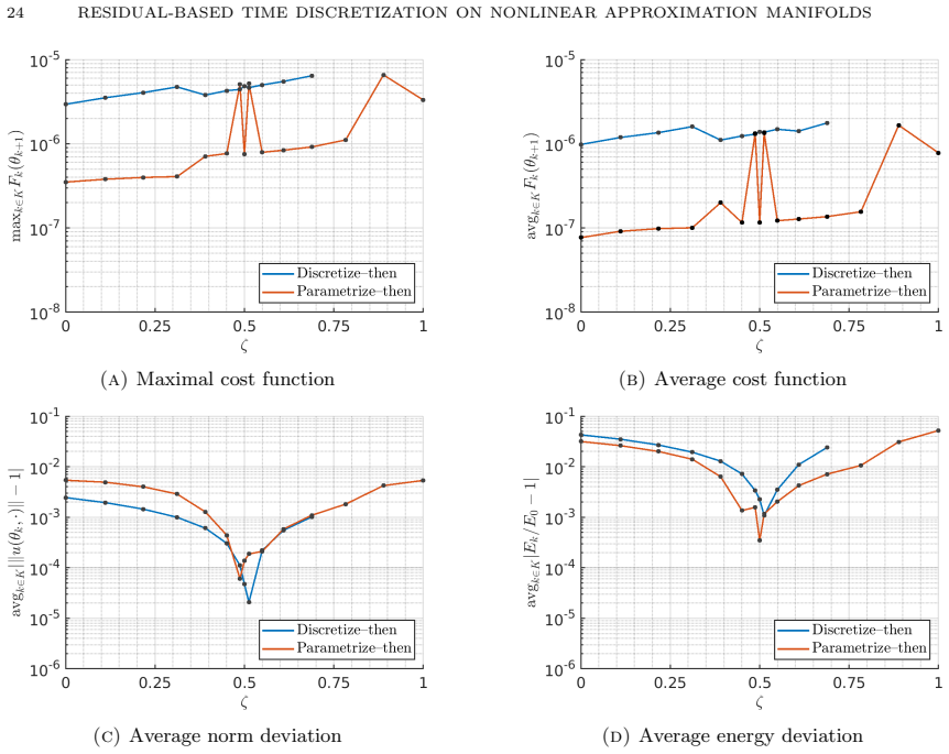
[§7.3, Table 2] The numerical support for the claimed rates is mixed. In Table 2, the fitted exponent pu for ζ=1/2 is 1.33 (L=1), 1.60 (L=3), 1.46 (L=5), and 2.09 (L=7) for parametrize-then, while for discretize-then it is 0.93, 1.14, 0.60, and −0.34; the negative exponent means the norm deviation increases as h decreases. The paper's residual-dominance explanation is plausible, but these data do not confirm the h^2 prediction of Theorems 4.1/4.2. Report ρ/h separately for each h (as in Fig. 8) and state explicitly the h-range in which the asymptotic rate is claimed.

minor comments (4)

[§3.3.2, Eq. (3.8)] The condition ∇θ b = \vec v b is stated with \vec v: Ω→C^p, but \vec v may depend on θ. For complex parameters, clarify whether the gradients are Wirtinger derivatives or full real gradients; the notation is currently ambiguous.
[§4, after Eq. (4.3)] The constants c1, c2 are introduced separately from the notation c_s used in Theorems 4.1 and 4.2. A short definition of c_s with s=1,2 would improve readability.
[§7.3, Table 2] Please report R^2 or residual standard errors for the fitted exponents. Several rows have very small C_u and one negative exponent, so the fit quality is unclear without additional diagnostic information.
[§7, Reproducibility paragraph] The reproducibility statement would benefit from specifying the Matlab release and exact fminunc settings, and from giving the repository URL in a footnote with the access date.

Circularity Check

0 steps flagged · score 0.0 of 10

No significant circularity: the error bounds are conditional and the residual is a measured output, not a fitted constant.

full rationale

The derivation chain is self-contained. Theorem 4.1 and Theorem 4.2 are conditional statements proved from the definitions of the residual and the local truncation error: the global error recursion (4.5) is obtained by subtracting the exact ζ-method relation (4.4) from the residual-defined update, and the rest is a standard Lipschitz/one-sided Lipschitz/dissipativity argument. The quantity ρ = max ∥r_k(θ_{k+1},·)∥ entering the final bounds is the a posteriori residual attained by the optimization step, not a fitted parameter and not a renamed version of the error being predicted. Theorem 4.2's additional constants m, σ0, γ_n are hypotheses with a conditional conclusion; even if those hypotheses fail for the Gaussian manifolds of Section 5, that is an applicability/validity concern, not circularity. The cited prior work [18], [19], [20], and [29] supplies background, motivation, or a starting point, but the main bounds are proved in the manuscript rather than imported as unverified premises. The numerical experiments are benchmarked against exact representable dynamics and an analytical Fokker-Planck solution, so the validation is external rather than self-referential. No equation in the paper reduces to its own input by construction.

Assumptions & free parameters 4 free parameters · 7 assumptions · 0 invented entities

The theoretical error bounds rely on Lipschitz/dissipativity, regularity, and two strong uniform bounds for the parametrize-then case; no new entities are postulated. Experimental free parameters are heuristic choices, not part of the central claim. ζ and h are explicit method parameters, not hidden degrees of freedom.

free parameters (4)

initial Gaussian width a / a'_0 = a=1.5 (basic init), a'_0=1.5·a0 (refinement)
Chosen by hand in §5.3.2 for initialization; not fitted and not part of the theoretical claims.
double-well initial state parameters a*, ν* = a*≈0.4475, ν*≈1.8732
Determined numerically by minimizing the energy of a two-Gaussian antisymmetric state in Test 2 (§6); used only as an initial condition for the double-well experiment.
optimization tolerances and max iterations = 1e-8, MaxIterations=200
BFGS stopping criteria listed in §6; user-chosen, not fitted.
number of Gaussian basis functions L = 1,3,5,7 in experiments
User-chosen manifold dimension controlling expressiveness; not fitted and not part of the theorem.

assumptions (7)

domain assumption f is (globally) Lipschitz or one-sided Lipschitz/dissipative on H (Theorem 4.1)
Assumed in Theorem 4.1 (Lip)/(os-Lip)/(diss); not satisfied by Schrödinger operators with unbounded potentials on all of H; the paper does not restrict to a bounded set.
domain assumption Exact solution regularity ψ∈C^2 or C^3
Used in (4.3) and Lemma A.1 to bound local error; standard regularity assumption.
ad hoc to paper Uniform lower singular value bound (4.7) and uniform bound (4.6)
Introduced in Theorem 4.2 to control parameter increments; strong and unverified for Gaussian manifolds over C^p.
domain assumption Existence of global minimizers at each time step
The scheme defines θ_{k+1}=argmin; in practice only local minima are found; this is treated black-box in Remark 2.1.
domain assumption Bounded derivatives of u(θ) with γ_n finite over Θ
c'_s in Theorem 4.2 depends on sup over θ; may be infinite on unbounded parameter space.
standard math Gaussian integral formula (5.2) with branch choice
Reference [10]; standard complex Gaussian integration with Re(a)>0.
standard math ζ-quadrature local error bound (Lemma A.1)
Proved in Appendix A using trapezoidal error estimates; standard.

how reviews work

0 comments

Cite this review

Pith. "Pith review of Residual-Based Time Discretization on Nonlinear Approximation Manifolds: Analysis and Gaussian Applications." pith.science (2026). https://pith.science/paper/TDRH765H

@misc{pith2026260715086,
  author       = {Pith},
  title        = {Pith review of: Residual-Based Time Discretization on Nonlinear Approximation Manifolds: Analysis and Gaussian Applications},
  year         = {2026},
  howpublished = {\url{https://pith.science/paper/TDRH765H}},
  note         = {Machine review of arXiv:2607.15086}
}

abstract

We study time-discrete parametric approximations of evolution equations in Hilbert spaces based on residual minimization. The solution is represented by a parametrized ansatz belonging to a low-dimensional nonlinear manifold, and time stepping is performed by minimizing suitably defined residuals at each step. Two natural residual formulations are considered: discretization followed by parametrization of the evolution equation, and discretization of the Dirac--Frenkel variational principle governing the parameter dynamics. A unified error analysis is developed for both approaches within the family of $\zeta$-methods. The resulting bounds separate the effects of time discretization from those of residual minimization and yield first- and second-order convergence under Lipschitz, one-sided Lipschitz, and dissipativity assumptions. For the variational formulation, additional stability conditions involving the conditioning of the parametrization map arise naturally. The framework is applied to Gaussian approximation manifolds, for which residual norms and gradients admit explicit closed-form expressions when polynomial operators are involved. This enables efficient implementation without spatial discretization. Numerical experiments for time-dependent Schr\"odinger equations illustrate the theoretical convergence rates and the influence of residual accuracy on conservation properties.

Figures

Figures reproduced from arXiv: 2607.15086 by the authors.

**Figure 1.** Approximation of two types of wave packets by L = 3 Gaussians. The top and bottom row show the approximation of the single Gaussian ψ Ex.1 0 = N0e −(x−2)2 and of the excited state ψ Ex.2 0 = N0H2(x − 1)e −(x−1)2 , respectively, where N0 are normalization constants. The plots to the left show the approximation with steps (i)–(iii), and the plots to the right show the improvement with step (iv). We have considered th… view at source ↗

**Figure 2.** Contour plots of the position density |ψ(t, x)| 2 for the harmonic oscillator. The left plot shows the dynamics for the Gaussian initial data, the right plot for the excited initial condition with a three-Gaussian approximation. Test 2: Double-well (interference and splitting). The potential is a double-well V (t, x) = α4x 4 + α2x 2 , x ∈ R, t ∈ [0, 10]. Following [14, 9], we choose the values for the potential as … view at source ↗

**Figure 3.** Contour plots of the position density |ψ(t, x)| 2 for the double-well. The left plot shows the dynamics of the first excited state (two-Gaussian approximation), the right plot shows the superposition (six-Gaussian approximation). left-hand side of [PITH_FULL_IMAGE:figures/full_fig_p020_3.png] view at source ↗

Figures from the paper (8 more)

**Figure 4.** Figure 4: Evolution of a single Gaussian initial condition in a hyperbolic cosine potential using multi-Gaussian approximations. Step-size: h = 10−3 . Reproducibility: algorithmic parameters. All numerical experiments have been done using a unified Matlab code4 admitting the fol…

**Figure 5.** Figure 5: Discretize–then approach. Comparison of the attained residual and energy deviation of the evolution of a single initial Gaussian condition in a doublewell (left) and hyperbolic cosine (right) potential using L = 1, 3, 5, 7 Gaussian basis functions. The plots in the to…

**Figure 6.** Figure 6: Hyperbolic cosine potential with one initial Gaussian. The approximate solution u(θk, ·) is built from L = 3 Gaussians, whose θ–parameters are optimized for each time step tk. The four plots show the outcome for the maximal and averaged cost function Fk = ∥rk(θk+1, ·)…

**Figure 7.** Figure 7: Double-well potential with one initial Gaussian. The approximate solution u(θk, ·) is built from L = 3 Gaussians, whose θ–parameters are optimized for each time step tk. The plots show the time-averaged cost function Fk = ∥rk(θk+1, ·)∥ 2 as well as the averaged norm an…

**Figure 8.** Figure 8: Hyperbolic cosine potential: scaled maximal residual and norm deviation (maximum) in dependence of the step-size h. Only the cases ζ = 0 and ζ = 1 2 are shown. This example corresponds to a seven-Gaussian approximation (L = 7) [PITH_FULL_IMAGE:figures/full_fig_p025_8.png]

**Figure 9.** Figure 9: Attained squared residuals Fk(θk+1) = ∥rk(θk+1, ·)∥ 2 and the norm deviation in dependence of time for: (i) shifted second excited state of the harmonic oscillator potential with a three-Gaussian approximation (left column), (ii) six-Gaussian approximation in a double…

**Figure 10.** Figure 10: shows the evolution of a single Gaussian wave packet ψ0(x) = N0e −(x+1)2 in four different regimes: a) A = 0, b = 0, D = 0.02; b) A = 0.02, b = 0, D = 0; c) A = 0, b = 4/10 + sin(2πt), D = 0; d) A = 0.01, b = 4/10 + sin(2πt), D = 0.01. We recall that b) is the diffusi…

**Figure 11.** Figure 11: Squared L 2 -norm of the difference between the exact solution ψ(t, ·) and the numerical solution u(t, ·) for t ∈ [0, 10], corresponding to the example with A ̸= 0, b ̸= 0, D ̸= 0, see Figure 10d. References [1] William Anderson and Mohammad Farazmand. “Fisher informa…

Discussion (0). Continue with ORCID to comment.

Reference graph

Works this paper leans on

29 extracted references · 2 canonical work pages

[1]

Fisher information and shape-morphing modes for solving the Fokker-Planck equation in higher dimensions

William Anderson and Mohammad Farazmand. “Fisher information and shape-morphing modes for solving the Fokker-Planck equation in higher dimensions”. English. In:Appl. Math. Comput.467 (2024). Id/No 128489, p. 17.issn: 0096-3003.doi: 10.1016/j.amc.2023.128489

arXiv 2024
[2]

Preprint, arXiv:2505.11938 [math.NA] (2025)

Daan Bon, Benjamin Caris, and Olga Mula.Stable Nonlinear Dynamical Approximation with Dynamical Sampling. Preprint, arXiv:2505.11938 [math.NA] (2025). 2025.url: https: //arxiv.org/abs/2505.11938

arXiv 2025
[3]

Neural Galerkin schemes with active learning for high-dimensional evolution equations

Joan Bruna, Benjamin Peherstorfer, and Eric Vanden-Eijnden. “Neural Galerkin schemes with active learning for high-dimensional evolution equations”. English. In:J. Comput. Phys. 496 (2024). Id/No 112588, p. 22.issn: 0021-9991.doi: 10.1016/j.jcp.2023.112588

arXiv 2024
[4]

Sparse quadrature for high-dimensional integration with Gaussian measure

Peng Chen. “Sparse quadrature for high-dimensional integration with Gaussian measure”. English. In:ESAIM, Math. Model. Numer. Anal.52.2 (2018), pp. 631–657.issn: 0764-583X. doi: 10.1051/m2an/2018012

arXiv 2018
[5]

Sharp error bounds for the trapezoidal rule and Simpson’s rule

D. Cruz-Uribe and C. J. Neugebauer. “Sharp error bounds for the trapezoidal rule and Simpson’s rule”. English. In:JIPAM, J. Inequal. Pure Appl. Math.3.4 (2002). Id/No 49, p. 22.issn: 1443-5756.url: https://eudml.org/doc/123201

2002
[6]

Fast training of accurate physics-informed neural networks without gradient descent

Chinmay Datar et al. “Fast training of accurate physics-informed neural networks without gradient descent”. In:The Fourteenth International Conference on Learning Representations. 2026.url: https://openreview.net/forum?id=3VdSuh3sie

2026
[7]

Davis and Philip Rabinowitz.Methods of numerical integration.English

Philip J. Davis and Philip Rabinowitz.Methods of numerical integration.English. Corrected reprint of the 1984 2nd ed. Mineola, NY: Dover Publications, 2007.isbn: 978-0-486-45339-2

1984
[8]

Mi-Song Dupuy, Virginie Ehrlacher, and Cl´ ement Guillot.Low-complexity approximations with least-squares formulation of the time-dependent Schr¨ odinger equation. 2025. arXiv: 2509. 13005[math.AP].url: https://arxiv.org/abs/2509.13005

arXiv 2025

Show all 29 references

[9]

to appear at Num

Michael Feischl et al.Regularized dynamical parametric approximation. to appear at Num. Math. 2026.url: https://arxiv.org/abs/2403.19234

2026
[10]

Folland.Harmonic analysis in phase space

Gerald B. Folland.Harmonic analysis in phase space. English. Vol. 122. Ann. Math. Stud. Princeton, NJ: Princeton University Press, 1989.isbn: 0-691-08528-5; 0-691-08527-7.doi: 10.1515/9781400882427. REFERENCES 31

1989 doi
[11]

Real time evolution with neural-network quantum states

Irene L´ opez Guti´ errez and Christian B. Mendl. “Real time evolution with neural-network quantum states”. In:Quantum6 (Jan. 2022), p. 627.issn: 2521-327X.doi: 10.22331/q- 2022-01-20-627.url: https://doi.org/10.22331/q-2022-01-20-627

2022 doi
[12]

Raising and lowering operators for semiclassical wave packets

George A. Hagedorn. “Raising and lowering operators for semiclassical wave packets”. Eng- lish. In:Ann. Phys.269.1 (1998), pp. 77–104.issn: 0003-4916.doi: 10.1006/aphy.1998.5843

1998
[13]

Time dependent variational approach to semiclassical dynamics

Eric J. Heller. “Time dependent variational approach to semiclassical dynamics”. In:The Journal of Chemical Physics64.1 (Jan. 1976), pp. 63–73.issn: 0021-9606.doi: 10.1063/1. 431911

1976 doi
[14]

Variational Approach for Linearly Dependent Moving Bases in Quan- tum Dynamics: Application to Gaussian Functions

Lo ¨ ıc Joubert-Doriol. “Variational Approach for Linearly Dependent Moving Bases in Quan- tum Dynamics: Application to Gaussian Functions”. In:Journal of Chemical Theory and Computation18.10 (2022). PMID: 36166838, pp. 5799–5809.doi: 10.1021/acs.jctc.2c00461

2022 doi
[15]

Jozef Kaˇ cur.Method of Rothe in evolution equations. English. Vol. 80. Teubner-Texte Math. Teubner, Leipzig, 1985

1985
[16]

The matrix singularity problem in the time-dependent variational method

Kenneth G. Kay. “The matrix singularity problem in the time-dependent variational method”. In:Chemical Physics137.1 (1989), pp. 165–175.issn: 0301-0104.doi: https://doi.org/10. 1016/0301-0104(89)87102-2

1989
[17]

Simen Kvaal et al.No need for a grid: Adaptive fully-flexible gaussians for the time-dependent Schr¨ odinger equation. 2023. arXiv: 2207.00271[quant-ph]

2023 arXiv
[18]

Computing quantum dynamics in the semiclassical regime

Caroline Lasser and Christian Lubich. “Computing quantum dynamics in the semiclassical regime”. English. In:Acta Numerica29 (2020), pp. 229–401.issn: 0962-4929.doi: 10.1017/ S0962492920000033

2020
[19]

Various variational approximations of quantum dynam- ics

Caroline Lasser and Chunmei Su. “Various variational approximations of quantum dynam- ics”. In:J. Math. Phys.63.7 (2022). Id/No 072107, p. 22.issn: 0022-2488.doi: 10.1063/5. 0088265

2022 doi
[20]

Christian Lubich.From quantum to classical molecular dynamics: reduced models and nu- merical analysis.English. Zur. Lect. Adv. Math. Z¨ urich: European Mathematical Society (EMS), 2008.isbn: 978-3-03719-067-8.doi: 10.4171/067

2008 doi
[21]

On variational approximations in quantum molecular dynamics

Christian Lubich. “On variational approximations in quantum molecular dynamics”. English. In:Math. Comput.74.250 (2005), pp. 765–779.issn: 0025-5718.doi: 10.1090/S0025-5718- 04-01685-0

2005 doi
[22]

Christian Lubich and J¨ org Nick.Regularized dynamical parametric approximation of stiff evolution problems. 2025. arXiv: 2501.12118[math.NA]

2025 arXiv
[23]

Physics-informed neural networks: A deep learning framework for solving forward and inverse problems involving nonlinear partial dif- ferential equations

M. Raissi, P. Perdikaris, and G.E. Karniadakis. “Physics-informed neural networks: A deep learning framework for solving forward and inverse problems involving nonlinear partial dif- ferential equations”. In:Journal of Computational Physics378 (2019), pp. 686–707.issn: 0021-99...

2019 doi
[24]

Quantum dynamics simulations using Gaussian wavepackets: the vMCG method

G.W. Richings et al. “Quantum dynamics simulations using Gaussian wavepackets: the vMCG method”. In:International Reviews in Physical Chemistry34.2 (2015), pp. 269–308. doi: 10.1080/0144235X.2015.1051354

2015
[25]

Simulation of a hydrogen atom in a laser field using the time-dependent variational principle

Keefer Rowan et al. “Simulation of a hydrogen atom in a laser field using the time-dependent variational principle”. In:Phys. Rev. E101 (2 Feb. 2020), p. 023313.doi: 10.1103/PhysRevE. 101.023313

2020 doi
[26]

Simon Elias Schrader et al.Rothe’s Method for Quantum Dynamics in Atoms and Molecules with Gaussian Wavepackets. 2026. arXiv: 2606 . 20947[physics.chem-ph].url: https : / / arxiv.org/abs/2606.20947

2026 arXiv
[27]

Time evolution as an optimization problem: The hydrogen atom in strong laser fields in a basis of time-dependent Gaussian wave packets

Simon Elias Schrader et al. “Time evolution as an optimization problem: The hydrogen atom in strong laser fields in a basis of time-dependent Gaussian wave packets”. In:The Journal of Chemical Physics161.4 (July 2024), p. 044105.issn: 0021-9606.doi: 10.1063/5.0213576

2024 doi
[28]

On Hagedorn wavepackets associated with different Gaussians

Jiˇ r ´ ı J. L. Van ´ ıˇ cek and Zhan Tong Zhang. “On Hagedorn wavepackets associated with different Gaussians”. In:Journal of Physics A: Mathematical and Theoretical58.085303 (2025).doi: 10.1088/1751-8121/adb083

2025 doi
[29]

Preprint, arXiv:2404.01145 [math.NA] (2024)

Huan Zhang et al.Sequential-in-time training of nonlinear parametrizations for solving time- dependent partial differential equations. Preprint, arXiv:2404.01145 [math.NA] (2024). 2024. url: https://arxiv.org/abs/2404.01145

2024 arXiv

Pith tools

Reviewed August 2, 2026 · model on record in the stance chip above.

[1] [1]

Fisher information and shape-morphing modes for solving the Fokker-Planck equation in higher dimensions

William Anderson and Mohammad Farazmand. “Fisher information and shape-morphing modes for solving the Fokker-Planck equation in higher dimensions”. English. In:Appl. Math. Comput.467 (2024). Id/No 128489, p. 17.issn: 0096-3003.doi: 10.1016/j.amc.2023.128489

arXiv 2024

[2] [2]

Preprint, arXiv:2505.11938 [math.NA] (2025)

Daan Bon, Benjamin Caris, and Olga Mula.Stable Nonlinear Dynamical Approximation with Dynamical Sampling. Preprint, arXiv:2505.11938 [math.NA] (2025). 2025.url: https: //arxiv.org/abs/2505.11938

arXiv 2025

[3] [3]

Neural Galerkin schemes with active learning for high-dimensional evolution equations

Joan Bruna, Benjamin Peherstorfer, and Eric Vanden-Eijnden. “Neural Galerkin schemes with active learning for high-dimensional evolution equations”. English. In:J. Comput. Phys. 496 (2024). Id/No 112588, p. 22.issn: 0021-9991.doi: 10.1016/j.jcp.2023.112588

arXiv 2024

[4] [4]

Sparse quadrature for high-dimensional integration with Gaussian measure

Peng Chen. “Sparse quadrature for high-dimensional integration with Gaussian measure”. English. In:ESAIM, Math. Model. Numer. Anal.52.2 (2018), pp. 631–657.issn: 0764-583X. doi: 10.1051/m2an/2018012

arXiv 2018

[5] [5]

Sharp error bounds for the trapezoidal rule and Simpson’s rule

D. Cruz-Uribe and C. J. Neugebauer. “Sharp error bounds for the trapezoidal rule and Simpson’s rule”. English. In:JIPAM, J. Inequal. Pure Appl. Math.3.4 (2002). Id/No 49, p. 22.issn: 1443-5756.url: https://eudml.org/doc/123201

2002

[6] [6]

Fast training of accurate physics-informed neural networks without gradient descent

Chinmay Datar et al. “Fast training of accurate physics-informed neural networks without gradient descent”. In:The Fourteenth International Conference on Learning Representations. 2026.url: https://openreview.net/forum?id=3VdSuh3sie

2026

[7] [7]

Davis and Philip Rabinowitz.Methods of numerical integration.English

Philip J. Davis and Philip Rabinowitz.Methods of numerical integration.English. Corrected reprint of the 1984 2nd ed. Mineola, NY: Dover Publications, 2007.isbn: 978-0-486-45339-2

1984

[8] [8]

Mi-Song Dupuy, Virginie Ehrlacher, and Cl´ ement Guillot.Low-complexity approximations with least-squares formulation of the time-dependent Schr¨ odinger equation. 2025. arXiv: 2509. 13005[math.AP].url: https://arxiv.org/abs/2509.13005

arXiv 2025