REVIEW 4 major objections 4 minor 40 references
Time lag in cosmic-ray modulation and global properties of the Solar Cycle
T0 review · 4 major / 4 minor · reviewed 2026-08-14 · deepseek-v4-flash
Pith's one-line read The paper reports a best-fit lag of 8.1 months for space-borne proton data and about 6 months from neutron monitors, arguing the delay reflects heliospheric propagation time.
desk verdict A conference status report that overclaims an unsupported 'first global characterization' while delivering only a repeated 8.1-month fit and a preliminary ~6-month correlation peak. read the letter →
The pith
A machine-rendered reading of the paper's core claim, the machinery that carries it, and where it could break.
The reading
What carries the argument
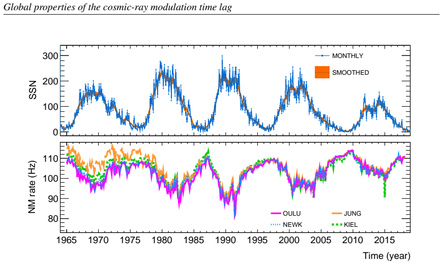
The central object is the retarded solar-input lag $\Delta T$, inserted into the transport model through relations such as $\kappa_0(t)=a+b\log(\hat{S}(t-\Delta T))$ and a retarded tilt angle $\hat{\alpha}(t-\Delta T)$. On the data side, the correlative method scans a single shift $\Delta T$ that maximizes the Pearson correlation between the neutron-monitor-derived modulation potential $\varphi(t)$ and the smoothed sunspot number, with $\varphi(t)$ obtained by inverting neutron-monitor rates via the force-field approximation, a mapping from a modulated spectrum to a single potential parameter. These two uses of the same parameter — one in a full transport fit, one in a direct correlation scan — carry the paper's quantitative claims.
What would settle it
Estimate the correlation-peak lag separately for each of the five solar cycles (or for each 22-year polarity epoch) from the same neutron-monitor data; if the peak lags differ by more than the statistical uncertainty, the single global lag reported here is an average artifact rather than a physical constant.
Extended reading notes
Core claim
Using a stochastic transport model with retarded solar inputs, the paper reaffirms a best-fit time lag of 8.1 months when fitting proton spectra from space-borne detectors between 2000 and 2012 under negative solar polarity. A separate correlative analysis converts neutron-monitor counting rates into the modulation potential $\varphi(t)$ through the force-field approximation, then scans the shift $\Delta T$ that maximizes the correlation between $\varphi(t)$ and the smoothed sunspot number $\hat{S}(t-\Delta T)$; this yields a peak lag of about 6 months over the 1964–2019 interval covering five solar cycles. The paper claims these values are consistent with an expected heliospheric propagation delay of 0.5–1 year, and it shows that a model with zero lag describes the proton data noticeably worse. It also reports that the delayed model does not reproduce the post-2013 ($A>0$) space-borne proton data well, which the authors take as evidence that a unique, constant lag may be insufficient.
Load-bearing premise
The result depends on the assumption that one single delay value, chosen to maximize the correlation between neutron-monitor-derived modulation and smoothed sunspot number, genuinely captures the physical lag across all five solar cycles — rather than being an average of different lags or an artifact of the conversion from counting rates to modulation potential.
Editorial extensions
If this is right
- Predictive models of cosmic-ray radiation near Earth should incorporate a delay of roughly half a year to eight months between solar activity and the modulated flux.
- The 1964–2019 neutron-monitor result provides a multi-cycle baseline against which future lag measurements at different energies can be compared.
- The discrepancy with post-2013 proton data implies that a single constant lag is insufficient, pointing toward cycle- or polarity-dependent lag values.
- A confirmed lag of this size constrains the effective size and flow speed of the heliospheric bubble, since the delay is interpreted as the transit time of solar-wind disturbances.
Reading between the lines
- The difference between the 8.1-month proton lag and the roughly 6-month neutron-monitor lag may reflect an energy or rigidity dependence: neutron monitors sample higher-rigidity particles than the proton data, so a systematic decrease of lag with rigidity would be a natural test of transport models.
- If the lag is truly cycle-dependent, then treating the correlation peak as a single global number will smear out the lag's relation to the 22-year magnetic polarity cycle; a natural extension is to fit the lag within each polarity epoch and look for a sign reversal.
- The force-field conversion of neutron-monitor rates to $\varphi$ assumes a particular local interstellar spectrum; redoing the analysis with different published LIS models would quantify how much of the 6-month peak is physical versus model-dependent.
Signed reviews
Editorial analysis
A structured set of objections, weighed in public.
Referee Report
Summary. The paper (arXiv:1908.01598, a proceedings contribution to ICRC2019) sets out to determine the time lag between solar activity, as proxied by the sunspot number, and the modulation of Galactic cosmic rays, and to characterize how this lag varies with solar cycle and particle energy. The authors first revisit their earlier stochastic transport model of heliospheric propagation, in which the time lag ΔT appears as a free parameter (together with diffusion-normalization constants a and b) relating diffusion coefficients to retarded solar inputs; refitting space-borne proton data over 2000–2012 (A<0 polarity) yields a best-fit lag of 8.1 months, as shown in Figure 1. They then describe a complementary approach using neutron monitor (NM) data from four stations over 1964–2019, converting NM rates into a modulation potential φ(t) under a force-field approximation, and determining the lag as the shift that maximizes the correlation between φ(t) and the smoothed sunspot number Ŝ(t−ΔT). For the full five-cycle interval, this correlation peaks at approximately 6 months (Figure 3). The abstract claims that this constitutes 'the first global characterization of the time lag evolution over the solar cycles and its energy dependence,' but the body of the paper, in the final paragraph of Section 3, explicitly states that the global analysis of lag dependence on solar-cycle phase, cycle number, and 22-year polarity is still being performed and will be published in a forthcoming paper.
Significance. A true global, cycle-resolved and energy-resolved determination of the cosmic-ray modulation time lag would be a valuable input for predictive radiation-dose models and for understanding heliospheric transport. The paper does assemble a large collection of space-borne and ground-based datasets, and it is transparent about the provisional character of the results, even noting a known disagreement with A>0 data in Figure 1. However, the only concrete quantitative outputs—an 8.1-month fit for one polarity epoch and a ~6-month correlation-peak average over five cycles—do not constitute the global characterization claimed in the abstract. The paper reads as a status report rather than a completed analysis; if the deferred global analysis were included and validated, the work could be significant, but as it stands the central claim is unsupported.
major comments (4)
- [Abstract and Section 3 (final paragraph)] The abstract states: 'In this work, we are perform the first global characterization of the time lag evolution over the solar cycles and its energy dependence.' Yet the final paragraph of Section 3 says: 'Using a generalized version of this method, we are now performing a global analysis based on the lag dependence on the solar cycles, or in the different phases of the 11-year activity cycles, or its dependence upon the 22-year cycle of magnetic polarity. The results will be presented at the conference and published in a forthcoming paper.' This is an explicit in-text statement that the global, cycle-resolved, energy-resolved characterization announced in the abstract is not contained in this manuscript. The only new quantitative result presented is a single scalar lag of about 6 months averaged over 1964–2019, with no cycle-by-cycle or energy-dependent breakdown. The headline claim is therefore unsupported by the manuscript's content.
- [Section 2 (Eq. 1 and Fig. 1)] The 8.1-month lag is not measured independently; it is the best-fit value of the free parameter ΔT in the authors' own transport model, with a and b also free parameters (k0(t) = a + b log Ŝ(t − ΔT)). Furthermore, the fit is restricted to 2000–2012 data during A<0 polarity, as the authors state. Figure 1 itself shows that the delayed model does not reproduce the post-reversal A>0 period after 2013, a discrepancy acknowledged in the text ('the predictions for the A>0 period do not agree well with the AMS data'). This single-polarity, single-phase fit cannot support a global characterization of lag evolution; it is a model-dependent fit output for one polarity epoch.
- [Section 3 (Fig. 3 and correlative method)] The ~6-month lag is obtained by maximizing the correlation between the NM-derived modulation potential φ(t) and the smoothed SSN Ŝ(t−ΔT) over the full 1964–2019 interval. This procedure assumes a single scalar lag applies across five solar cycles and multiple polarity reversals. The authors themselves note that 'dependence on the solar cycle have been noted [3, 38, 39, 40]', which undermines the adequacy of a single global scalar lag. In addition, the φ(t) series are constructed using a force-field approximation and per-station normalization factors; no systematic uncertainties from these modeling steps are propagated into the quoted lag value. The result is therefore at best an unweighted average over heterogeneous epochs, not a characterization of lag evolution.
- [Abstract and Section 3] The abstract promises 'energy dependence' of the time lag, but no energy-resolved analysis is presented anywhere in the manuscript. The NM data are energy-integrated by construction, as the text acknowledges, and the space-borne analysis is limited to a single broad energy bin around 1 GeV in Figure 1. Thus the energy-dependence claim has no supporting quantitative result in the paper.
minor comments (4)
- [Abstract] The phrase 'we are perform the first global characterization' is ungrammatical; it should be 'we perform' or 'we report on'. Similar grammatical slips appear elsewhere (e.g., 'If we regarding the heliosphere' in Section 2).
- [Section 3 (Fig. 3)] The caption of Figure 3 states 'the correlation coefficient functions ρ(ΔT) are shown for various NM stations (left)', but the left panel appears to show a single curve or multiple curves that are not individually labeled for each station. The exact peak location and its uncertainty for each station are not stated; only 'about six months' is given in the text.
- [Section 3 (text after Eq. 3.2)] The sentence 'The last factor Jj(t,E) represents the modulated energy spectra of all contributing GCR species' is clear, but the preceding factorized form Y^d_j = V^d F^d_j is introduced without defining the superscript d consistently for V and F; this may confuse readers following the detector-response derivation.
- [Table 1] The cutoff rigidity for Jungfraujoch is listed as 4500 MV, which is unusually high for a station at 3570 m altitude; if this is correct, a brief justification or reference would be helpful, though it does not affect the main conclusions.
Circularity Check
No circularity: the lag values are openly estimated by fitting/correlation, and the unsupported 'global characterization' claim is a completeness issue, not a derivation that reduces to its input.
full rationale
The paper's quantitative lag values are presented as estimates, not as first-principles predictions. Section 2 states that in the transport model 'κ0(t) = a + b log(Ŝ(t−ΔT)), where a, b, and ΔT are free parameters', and the 8.1-month value is a best-fit result from a global fit over 2000–2012 A<0 data. Section 3 states that 'the resulting lag ΔT is determined as the parameter that maximizes the correlation between the modulation potential φ(t) (at epoch t) and the smoothed SSN Ŝ(t−ΔT)', and Fig. 3 reports the resulting peak at about 6 months. These are standard parameter-estimation procedures: the fitted value is the estimator's output, and the paper does not use that same fitted value to predict a separate quantity or to validate its model in a circular loop. The abstract's claim of performing the 'first global characterization of the time lag evolution over the solar cycles and its energy dependence' is not supported by the body—Section 3 explicitly says the global, cycle-resolved analysis 'will be presented at the conference and published in a forthcoming paper.' That is an overclaim or missing-support issue, not circularity. Self-citations such as [24] and [25] introduce the transport and NM-response models and an earlier 8.1-month fit, but the paper refits the lag with updated data, so the self-citations are not load-bearing in a way that forces the conclusion. No equation reduces to its own input, and no fitted parameter is renamed as a prediction. Therefore the circularity score is 0.
Assumptions & free parameters
free parameters (3)
- ΔT (time lag) =
8.1 months (space fit), ~6 months (NM correlation)
- a, b (diffusion normalization constants) =
not given in paper
- Per-station NM normalization factors =
not given in paper
assumptions (4)
- domain assumption Force-field approximation is adequate to convert NM counting rates to a single modulation potential φ at NM-response energies
- domain assumption Sunspot number is a good proxy for the solar magnetic activity that drives GCR modulation
- domain assumption A single retarded time shift ΔT in SSN and tilt angle captures the physical lag in the transport model
- domain assumption The heliosphere can be treated as a spherical bubble with wind speed 300-700 km/s giving ΔT ~0.5-1 year
Cite this review
Pith. "Pith review of Time lag in cosmic-ray modulation and global properties of the Solar Cycle." pith.science (2026). https://pith.science/paper/TEAYXQB7
@misc{pith2026190801598,
  author       = {Pith},
  title        = {Pith review of: Time lag in cosmic-ray modulation and global properties of the Solar Cycle},
  year         = {2026},
  howpublished = {\url{https://pith.science/paper/TEAYXQB7}},
  note         = {Machine review of arXiv:1908.01598}
}
read the original abstract
When entering the heliosphere, Galactic cosmic rays (GCRs) are influenced by magnetic turbulence and Solar wind disturbances, which cause the so-called "solar modulation" effect. Understanding the time-dependent relationship between the Sun's variability and GCR flux modulation is essential for the investigation of the GCR transport processes in the heliosphere, as well as for the establishment of predictive models of GCR radiation in the interplanetary space. The known anti-correlation between GCR flux and sunspot number appears to be delayed by several months, but the origin of such a time lag is unclear. In this work, we are perform the first global characterization of the time lag evolution over the solar cycles and its energy dependence. We made use of a large collection of time-resolved data, both from space missions and ground based observatories. Since the long-term variation of the GCR flux originates by a combination of several physics processes, the investigation presented here may reveal important aspects of the GCR transport in the heliospheric plasma.
Figures


Reference graph
Works this paper leans on
- [1]
-
[2]
Usoskin, I.G., et al., J. Geophys. Res. 103, 9567 (1998)
work page 1998
-
[3]
Ross, E., & Chaplin, W., Sol. Phys. 294, 8 (2019)
work page 2019
-
[4]
Kuznetsov, N. V ., Popova, H., Panasyuk, M. I.,J. Geophys. Res. Space Phys., 122, 1463â ˘A¸ S1472 (2017)
work page 2017
-
[5]
Matthia, D., Berger, T., Mrigakshi, A. I., Reitz, G., Adv. Space Res. 51, 329-338 (2013)
work page 2013
- [6]
-
[7]
O’Neill, P. M., Golge, S., Slaba, T. C., NASA/TPâ ˘A¸ S2015â˘A¸ S218569 (2015)
work page 2015
- [8]
Show all 40 references
-
[9]
Kühl, P., Gómez-Herrero, R., Heber, B., Sol. Phys. 291, 965-974 (2016)
2016
-
[10]
Abe, K., et al., Phys. Rev. Lett. 108, 051102 (2012); Abe, K., et al., Phys. Lett. B 670, 103 (2008)
2012
-
[11]
Aguilar, M., et al., Phys. Rev. Lett. 121, 051101 (2018)
2018
-
[12]
Aguilar, M., et al., Phys. Rev. Lett. 114, 171103 (2015)
2015
-
[13]
Aguilar, M., et al., Phys. Rev. Lett. 115, 211101 (2015)
2015
-
[14]
Adriani, O., et al., Astrophys. J. 765, 91, (2013)
2013
-
[15]
Martucci, M., et al., Astrophys. J. 854, L2 (2018)
2018
-
[16]
Clette, F., & Lefèvre, L., Sol. Phys. 291, 2629-2651 (2016)
2016
-
[17]
T., Space Sci
Hoeksema, J. T., Space Sci. Rev. 72, 137-148 (1995)
1995
-
[18]
Tomassetti, N., et al., Phys. Rev. Lett. 121, 251104 (2018)
2018
-
[19]
Tomassetti, N., Phys. Rev. D 92, 081301 (2015)
2015
-
[20]
Tomassetti, N., Astrophys. J. Lett. 815, L1 (2015)
2015
-
[21]
Tomassetti, N., Astrophys. J. 752, L13 (2012)
2012
-
[22]
Feng, J., Tomassetti, N., Oliva, A., Phys. Rev. D 94, 123007 (2016)
2016
-
[23]
C., et al., Astrophys
Cummings, A. C., et al., Astrophys. J. 831, 18 (2016)
2016
-
[24]
Tomassetti, N., Orcinha, M., Barão, F., Bertucci, B., Astrophys. J. Lett. 849, 32 (2017)
2017
-
[25]
Tomassetti, N., Phys. Rev. D 96, 103005 (2017)
2017
-
[26]
Kappl, R., Comp. Phys. Comm. 207 (2016) 386-399 6 Global properties of the cosmic-ray modulation time lag
2016
-
[27]
D., Effenberger, F., Space Sci Rev (2017)
Strauss, R. D., Effenberger, F., Space Sci Rev (2017)
2017
-
[28]
T., Liu, Y ., Zhao, J.,Astrophys
Sun, X., Hoeksema, J. T., Liu, Y ., Zhao, J.,Astrophys. J. 798, 114 (2015)
2015
-
[29]
Dorman, L., 2009, V ol. 358. Springer, 2009. ISBN: 978-1-4020-9238-1
2009
-
[30]
& Astrophys
Ghelfi, A., Barao, F., Derome, L., Maurin, D., Astron. & Astrophys. 591, A94 (2016)
2016
-
[31]
G., Bazilevskaya, G
Usoskin, I. G., Bazilevskaya, G. A., Kovaltsov, G. A., J. Geophys. Res. 116, A2 (2011)
2011
-
[32]
F., & Shea, M
Smart, D. F., & Shea, M. “P.” A., Adv. Space Res. 36, 2012-2020 (2005)
2005
-
[33]
Tomassetti, N., Phys. Rev. C 92, 045808 (2015)
2015
-
[34]
Cheminet, A., et al., J. Geophys. Res. 118, 7488-7496 (2013)
2013
-
[35]
34th ICRC - The Hague, PoS 225 (2015)
Steigies, C., Proc. 34th ICRC - The Hague, PoS 225 (2015)
2015
-
[36]
Space Res
Mavromichalaki, H., et al., Adv. Space Res. 47 2210-2222 (2011)
2011
-
[37]
R., Yuan, Q., Wei, D
Zhu, C. R., Yuan, Q., Wei, D. M., Astrophys. J. 863, 119 (2018)
2018
-
[38]
& Badruddin, Sol
Aslam, O.P.M. & Badruddin, Sol. Phys. 290, 2333-2353 (2015)
2015
-
[39]
K., & Mishra, A
Mishra, V . K., & Mishra, A. P.,Sol. Phys. 293, 141 ((2018))
2018
-
[40]
A., & Suslov, A
Nymmik, R. A., & Suslov, A. A., Adv. Space Res. 16, 9217-9220 (1995) 7
1995
Reviewed August 14, 2026 · model on record in the stance chip above.
Discussion (0). Continue with ORCID to comment.