REVIEW 3 major objections 6 minor 85 references
Vakonomic Fluids
T0 review · 3 major / 6 minor · reviewed 2026-08-04 · deepseek-v4-flash
Pith's one-line read Forcing every variation to respect the discretized velocity constraint yields fluid paths that are true geodesics, conserving energy, enstrophy-like invariants, and circulation to machine precision.
desk verdict Clean vakonomic Lax derivation and a strong discrete Kelvin theorem, but the abstract oversells conservation and the continuum limit is unproven. read the letter →
The pith
A machine-rendered reading of the paper's core claim, the machinery that carries it, and where it could break.
The reading
What carries the argument
The load-bearing object is the vakonomic variational principle applied to the right-invariant K-metric restricted to the distribution D_R = {XR : X ∈ im(A-bar)} in T SO(F). Lagrange–d'Alembert lets variations leave the distribution and therefore requires an ad hoc ambient-metric choice; the vakonomic principle instead confines the whole variation family to admissible paths, and the stationarity condition then closes as the Lax equation dZ/dt = [Z^#, Z]. The sharp operator # = A-bar K^-1 A-bar* is defined solely from the discrete advection operator and the velocity mass matrix K, so no metric information from outside the constraint space is needed — the heart of the paper's self-consistency c
What would settle it
Run the reset-free scheme on a Taylor–Green vortex at 32→64→128→256 resolution and measure the L^2 error of the vorticity field against the exact steady solution; if the error does not shrink at a stable order, the dynamics are structure-preserving but not a discretization of Euler. Alternatively, run a two-dipole leapfrogging experiment with resetting disabled: if tr(Z^2) and tr(Z^4) hold to machine precision while the vortex trajectories visibly miss the point-vortex prediction, then the exactly conserved structure is not the one that carries the fluid physics.
Extended reading notes
Core claim
Set up discrete fluid motion as a path R(t) in SO(F) whose body velocity X = dR/dt R^-1 is constrained to the image im(A-bar) of a discrete advection operator; because im(A-bar) is not closed under the matrix commutator, this is a genuine nonholonomic constraint. The paper proves that stationarity of the kinetic-energy action under variations that keep the family inside the constraint distribution — the vakonomic principle, as opposed to Lagrange–d'Alembert — is equivalent to a coadjoint evolution on so(F)* that reads, after the Frobenius identification, as the matrix Lax equation dZ/dt = [Z^#, Z], with sharp map # = A-bar K^-1 A-bar* built only from constraint-space data. This evolution is
Load-bearing premise
The whole construction rests on the premise that the constrained rotation-matrix dynamics actually approaches the incompressible Euler equations as the grid is refined — the paper proves exact structure preservation but explicitly leaves the convergence of its discrete Lie algebra to the divergence-free vector fields open; if that convergence fails, the method is a self-consistent toy rather than a discretization of Euler flow.
Editorial extensions
If this is right
- Discrete ideal-fluid simulations become exactly isospectral: enstrophy- and helicity-like Casimirs no longer drift, removing a common source of spurious energy cascades in long runs.
- One source of arbitrariness vanishes: unlike Lagrange–d'Alembert discretizations, the equations carry no free 'ambient metric' — only the choice of function space, velocity space, and mass matrix.
- The low-rank Clebsch form reduces the per-step cost from O(F^2) to O(mF), making exactly structure-preserving ideal-fluid simulation practical on standard FEEC/B-spline and triangle-mesh grids without ever assembling a dense matrix.
- The conserved discrete circulation is stronger than the weak circulation of earlier projected-Lax schemes: it holds for every loop transported by the flow, not merely in a projected sense.
- The same variational framework extends to semidirect-product physics — stratified Boussinesq flow is demonstrated, and the authors sketch shallow-water, compressible, and MHD variants.
Reading between the lines
- My inference: the reset step, which the paper needs to curb dispersion, breaks the exact conservation the construction advertises; a natural testable extension is the paper's own suggestion of double-bracket dissipation, which would limit dispersion while keeping Casimirs exactly conserved.
- My inference: the advertised clean separation of time-integration drift from resetting drift is only implicit in the figures; a reset-free diagnostic run that logs tr(Z^2) and tr(Z^4) every step would settle how much of the observed dissipation is actually the reset's doing.
- My inference: the circulation theorem's physical content depends on how faithfully the Lie-algebraic closure of im(A-bar) represents real material loops; a coarse-mesh reset-free run against analytical point-vortex or shielded-vortex trajectories would quantify that fidelity.
- My inference: the m = d choice of Clebsch pairs sets a fixed rank for Z, and the paper gives no rank-robustness test; sweeping m while monitoring the reconstructed velocity would show whether truncation in the low-rank ansatz is a source of error comparable to the discretization error.
Editorial analysis
A structured set of objections, weighed in public.
Referee Report
Summary. The paper introduces a finite-dimensional discretization of the incompressible Euler equations based on a Koopman representation of volume-preserving diffeomorphisms on half-densities. The discretized velocity constraint X ∈ im(Ā) is nonholonomic, and the authors treat it with the vakonomic variational principle, obtaining a reduced Lie–Poisson system in Lax form, Eq. (6.12): Ż = [Z^#, Z]. They show this system is isospectral, hence preserves Casimir invariants, and satisfies a discrete analogue of Kelvin's circulation theorem. A low-rank Clebsch momentum-map representation reduces the computational cost from O(F^2) to O(mF), and a Lie-trapezoidal time integrator preserves energy and the coadjoint orbit in the reset-free case. The practical algorithm includes a periodic resetting procedure to control dispersion. Numerical experiments include Taylor–Green vortex convergence, invariant checks, shielded and leapfrogging vortices, flows on surfaces, a 3D trefoil knot, and a Boussinesq Rayleigh–Taylor simulation.
Significance. The core geometric derivation is clean and largely self-contained: Theorem 6.1 derives the coadjoint equation from the vakonomic action, Lemma 6.1 gives the coadjoint action on so(F), and Theorem 8.1 shows the Clebsch ansatz satisfies the Lax equation exactly. The integrator analysis in Theorem 9.1 is rigorous and the numerical experiments are extensive. If the discrete system were shown to converge to the Euler equations in the continuum limit, this would be an important contribution to structure-preserving fluid simulation. Even without such a convergence theorem, the Lax formulation, the low-rank momentum-map representation, and the numerical evidence of reduced dispersion are valuable. The paper is also commendably explicit about its open questions, especially the continuum-limit issue in Section 12.
major comments (3)
- [Section 12; Sections 5–6] The paper's central claim—that the vakonomic Lax system (6.12) is a discretization of the incompressible Euler equations (3.9)—is not established. Section 12 explicitly leaves open whether so(F) and im(Ā) converge to sdiff(M), and the numerical evidence in Fig. 12 is only for the steady Taylor–Green vortex. Without a consistency or convergence result for the general initial-value problem, Eq. (6.12) is a self-consistent isospectral flow on so(F) but not proven to approximate Eq. (3.9). I recommend either supplying such a result or reframing the contribution as a structure-preserving discrete fluid model whose relation to the Euler equations is empirical.
- [Abstract; Section 10.3; Section 11.1.1] The abstract's 'machine-precision satisfaction of Casimir invariants' is true only in the reset-free limit. Algorithm 6 includes resets, all production experiments use resets (Table 2), and Section 11.1.1 reports a 1.6% energy drop over 5 s for TGV with resets; Fig. 16 shows Casimir jumps at each reset. Since resetting is a non-Hamiltonian heuristic (Sec. 10.3.2), the headline conservation claim should be qualified to the reset-free integrator, and the practical algorithm should be presented as approximately structure-preserving with quantified drift.
- [Section 8; Section 12] The low-rank Clebsch ansatz (8.2) is exact on the invariant manifold rank(Z) ≤ 2m, but the paper does not quantify the approximation error for general initial data that are not low-rank, nor does it prove that the discrete analogue of the d−1 Clebsch-pair sufficiency of [83] holds in the finite-dimensional setting. The paper itself notes 'some variance in practice' (Sec. 12). This is not fatal, but it should be acknowledged explicitly in the main text rather than presenting the low-rank model as a closed reduced-order description with no approximation gap.
minor comments (6)
- [Section 6] Heading typo: 'Eqations' should be 'Equations'.
- [Section 5.4] The symbol V is used both for the finite element space and for its dimension. Use, e.g., dim V to avoid ambiguity.
- [Figure 15 / Table 2] The reset-frequency parameter α in Fig. 15 is not defined in the table or caption; clarify whether it is a step count or a time interval.
- [Section 10.3.1] The FTLE threshold S_f ≤ 1 is stated to 'consistently lead to good results' but no sensitivity analysis is provided; this is an empirical heuristic and should be labeled as such.
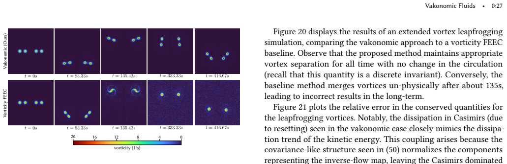
- [Section 11.1.2] The comparison baseline 'Vorticity FEEC' is reconstructed via Reset for Casimir diagnosis. Please explain why this reconstruction is faithful to the LdA dynamics; otherwise the comparison in Fig. 14 is difficult to interpret.
- [Section 7.1] The statement that LdA is 'not self-consistent' is normative; consider rewording to 'not variational in the same intrinsic sense' to avoid overstatement.
Circularity Check
Main Lax derivation is self-contained; the advertised discrete Kelvin theorem is a definitional restatement, and resetting plus the unproven continuum limit qualify the headline claims.
-
self definitional
[Section 6.3.2, Theorem 6.2 (after Eq. (6.12))]
"A time-dependent discrete loop Y(t) is said to be transported by the flow of X(t) if it satisfies the Lax equation Ÿ(t)=[X(t),Y(t)]. ... Given a covector Z∈so(F)*, the circulation of Z along the discrete loop Y∈so(F) is just the evaluation pairing ⟨Z|Y⟩. So, a path Z satisfies Kelvin's circulation law ... if the circulation ⟨Z(t)|Y(t)⟩=⟨Z(0)|Y(0)⟩ is independent of t for all loops Y ... satisfying the Lax equation Ÿ(t)=[X(t),Y(t)]."
The theorem states that Z satisfies Ż=[X,Z] iff ⟨Z|Y⟩ is constant for every Y with Ÿ=[X,Y]. Because 'transported' is defined as satisfying the Lax equation and 'circulation' is defined as the pairing, the proof reduces to d/dt⟨Z|Y⟩=⟨Ż+ad*_X Z|Y⟩, which is zero exactly when the Lax equation holds (using ad*_X Z=-[X,Z]). The advertised discrete Kelvin theorem is therefore a restatement of Lax-pair invariance, not an independent consequence derived from the variational principle. It adds no content beyond the isospectral structure already present in Eq. (6.12).
full rationale
The core derivation in Sections 3–6 is self-contained: the vakonomic action (6.7), Lagrange multiplier, and sharp map produce the coadjoint equation (6.9) and the Lax form (6.12) without assuming the target result. The claimed Lie–Poisson structure and Casimir preservation are direct mathematical consequences of the Lax/isospectral structure and the coadjoint-orbit-preserving integrator (Theorem 9.1), not fitted inputs. Numerical verifications are self-consistency checks of exact invariants plus external benchmarks such as Taylor–Green and point vortices, so they are not circular predictions. Two acknowledged limitations, the open continuum-limit question in Section 12 and the resetting procedure in Section 10.3, are not circularity: the former leaves the Euler-discretization claim conditional, and the latter explicitly breaks exact Casimir conservation in the implemented algorithm. Self-citations [70] and [71] are used for implementation choices and heuristics rather than to justify the central derivation. The only definitional circularity is the 'discrete Kelvin theorem,' which is a restatement of Lax-pair invariance.
Assumptions & free parameters
free parameters (4)
- Reset period =
Per-experiment: e.g., 2.29 s (TGV 128), 0.21 s (trefoil), 0.12 s (bunny); or FTLE-triggered
- FTLE reset threshold S_f =
S_f ≤ 1
- Number of Clebsch pairs m =
m = d (2 or 3)
- Time step Δt =
varies per experiment (Table 2)
assumptions (5)
- domain assumption The discrete Koopman representation imposes a nonholonomic constraint X ∈ im(Ā) that is the correct discrete analogue of the continuous constraint im(adv) ⊂ so(HD(M)).
- domain assumption The finite-dimensional sub-Riemannian structure (SO(F), D, ⟨·,·⟩_K) yields geodesics that converge to continuous Euler solutions in the continuum limit.
- domain assumption FEEC spaces give pointwise divergence-free velocity and exact Hodge decomposition, making V_div = {u | div(u)=0}.
- ad hoc to paper The low-rank Clebsch ansatz Z = 1/2 Σ (λ_a μ_a^T − μ_a λ_a^T) captures the relevant dynamics of the full Lax equation.
- standard math Standard results in variational calculus and sub-Riemannian geometry (e.g., [75]) justify the equivalence of vakonomic critical points and sub-Riemannian geodesics.
invented entities (2)
-
Discrete loop Y ∈ so(F) transported by the flow Ẏ=[X,Y]
-
Accumulated gravity half-density g
Cite this review
Pith. "Pith review of Vakonomic Fluids." pith.science (2026). https://pith.science/paper/TIR6SILI
@misc{pith2026260718312,
  author       = {Pith},
  title        = {Pith review of: Vakonomic Fluids},
  year         = {2026},
  howpublished = {\url{https://pith.science/paper/TIR6SILI}},
  note         = {Machine review of arXiv:2607.18312}
}
read the original abstract
We introduce a novel discretization of the incompressible Euler equations based on their interpretation as geodesic equations on the Lie group of volume-preserving diffeomorphisms. It is well known that encoding diffeomorphisms and their infinitesimal generators through a discretized Koopman representation places a nonholonomic constraint on discrete velocities, for which there is no consensus on a variational treatment. We show that taking the vakonomic perspective, as opposed to the usual perspective of Lagrange--d'Alembert, yields discrete fluid trajectories that remain geodesics on a (sub-)Riemannian manifold. In particular, the resulting vakonomic dynamics are Lie--Poisson and their solutions admit a discrete relabeling symmetry, leading to machine-precision satisfaction of Casimir invariants along with a discrete analogue of Kelvin's Circulation Theorem. Using an efficient momentum map representation based on low-rank Clebsch variables, we show that these vakonomic fluids behave stably and consistently even at low grid resolutions, leading to increased robustness and physical realism in the long term.
Figures


Figures from the paper (37 more)




Reference graph
Works this paper leans on
-
[83]
Yoshida,Clebsch parameterization: Basic properties and remarks on its applications, Journal of Mathematical Physics50(2009), no
Z. Yoshida,Clebsch parameterization: Basic properties and remarks on its applications, Journal of Mathematical Physics50(2009), no. 11, 113101
2009
-
[1]
Abanov and Boris Khesin,Infinite- Dimensional Nonholonomic and Vakonomic Systems, Jour- nal of Nonlinear Science36(2026), no
Alexander G. Abanov and Boris Khesin,Infinite- Dimensional Nonholonomic and Vakonomic Systems, Jour- nal of Nonlinear Science36(2026), no. 3, 67
2026
-
[2]
Al-Mohy and Nicholas J
Awad H. Al-Mohy and Nicholas J. Higham,Computing the Action of the Matrix Exponential, with an Applica- tion to Exponential Integrators, SIAM Journal on Scientific Computing33(2011), no. 2, 488–511. 35
2011
-
[3]
2, 281–354
Douglas Arnold, Richard Falk, and Ragnar Winther,Fi- nite element exterior calculus: from hodge theory to nu- merical stability, Bulletin of the American mathematical society47(2010), no. 2, 281–354
2010
-
[4]
Arnold,Finite Element Exterior Calculus, Soci- ety for Industrial and Applied Mathematics, Philadelphia, PA, 2018
Douglas N. Arnold,Finite Element Exterior Calculus, Soci- ety for Industrial and Applied Mathematics, Philadelphia, PA, 2018
2018
-
[5]
Arnold, Richard S
Douglas N. Arnold, Richard S. Falk, and Ragnar Winther, Finite element exterior calculus, homological techniques, and applications, Acta Numerica15(2006), 1–155
2006
-
[6]
1, 319–361 (fre)
Vladimir Arnold,Sur la g ´eom´etrie diff ´erentielle des groupes de Lie de dimension infinie et ses applications `a l’hydrodynamique des fluides parfaits, Annales de l’institut Fourier16(1966), no. 1, 319–361 (fre)
1966
-
[7]
Arnold, Valery V
Vladimir I. Arnold, Valery V. Kozlov, and Anatoly I. Neishtadt,Basic Principles of Classical Mechanics, Math- ematical Aspects of Classical and Celestial Mechanics: Third Edition, Springer Berlin Heidelberg, Berlin, Heidel- berg, 2006, pp. 1–60
2006
Show all 85 references
-
[8]
5, 73–82
Omri Azencot, Mirela Ben-Chen, Fr ´ed´eric Chazal, and Maks Ovsjanikov,An Operator Approach to Tangent Vec- tor Field Processing, Computer Graphics Forum32(2013), no. 5, 73–82
2013
-
[9]
Graph.34 (2015), no
Omri Azencot, Maks Ovsjanikov, Fr ´ed´eric Chazal, and Mirela Ben-Chen,Discrete Derivatives of Vector Fields on Surfaces – An Operator Approach, ACM Trans. Graph.34 (2015), no. 3
2015
-
[10]
5, 237–246
Omri Azencot, Steffen Weißmann, Maks Ovsjanikov, Max Wardetzky, and Mirela Ben-Chen,Functional Fluids on Surfaces, Computer Graphics Forum33(2014), no. 5, 237–246
2014
-
[11]
G. K. Batchelor,An Introduction to Fluid Dynamics, Cambridge Mathematical Library, Cambridge University Press, 2000
2000
-
[12]
Werner Bauer and Franc ¸ois Gay-Balmaz,Towards a geo- metric variational discretization of compressible fluids: The rotating shallow water equations, Journal of Computa- tional Dynamics6(2019), no. 1, 1–37
2019
-
[13]
4, 511– 537
Werner Bauer and Franc ¸ois Gay-Balmaz,Variational in- tegrators for anelastic and pseudo-incompressible flows, Journal of Geometric Mechanics11(2019), no. 4, 511– 537
2019
-
[14]
Ferraro, David Mart ´ın de Diego, and Shreyas Bharadwaj,Discrete variational calculus for double-bracket dissipation, 2026
Anthony Bloch, Sebasti ´an J. Ferraro, David Mart ´ın de Diego, and Shreyas Bharadwaj,Discrete variational calculus for double-bracket dissipation, 2026
2026
-
[15]
Anthony M Bloch, John Baillieul, Peter E Crouch, Jer- rold E Marsden, and Dmitry Zenkov,Nonholonomic me- chanics and control, Interdisciplinary Applied Mathemat- ics, Springer New York, New York, 2015
2015
-
[16]
720, 1070–1088
R ¨udiger Brecht, Werner Bauer, Alexander Bihlo, Franc ¸ois Gay-Balmaz, and Scott MacLachlan,Variational integra- tor for the rotating shallow-water equations on the sphere, Quarterly Journal of the Royal Meteorological Society 145(2019), no. 720, 1070–1088
2019
-
[17]
Brunton, Marko Budi ˇsi´c, Eurika Kaiser, and J
Steven L. Brunton, Marko Budi ˇsi´c, Eurika Kaiser, and J. Nathan Kutz,Modern Koopman Theory for Dynamical Systems, SIAM Review64(2022), no. 2, 229–340
2022
-
[18]
Buffa, J
A. Buffa, J. Rivas, G. Sangalli, and R. V ´azquez,Isogeomet- ric Discrete Differential Forms in Three Dimensions, SIAM Journal on Numerical Analysis49(2011), no. 2, 818–844
2011
-
[19]
Buffa, G
A. Buffa, G. Sangalli, and R. V ´azquez,Isogeometric anal- ysis in electromagnetics: B-splines approximation, Com- puter Methods in Applied Mechanics and Engineering 199(2010), no. 17, 1143–1152
2010
-
[20]
2161, Springer, Cham, Switzerland, 2016
Annalisa Buffa and Giancarlo Sangalli,Isogeometric anal- ysis: a new paradigm in the numerical approximation of pdes: Cetraro, italy 2012, vol. 2161, Springer, Cham, Switzerland, 2016
2012
-
[21]
220, 1461–1486
Mari Paz Calvo, Arieh Iserles, and Antonella Zanna, Numerical Solution of Isospectral Flows, Mathematics of Computation66(1997), no. 220, 1461–1486
1997
-
[22]
Calvo, A
M.P. Calvo, A. Iserles, and A. Zanna,Runge-Kutta meth- ods for orthogonal and isospectral flows, Special Issue Celebrating the Centenary of Runge-Kutta Methods22 (1996), no. 1, 153–163
1996
-
[23]
Elena Celledoni, H ˚akon Marthinsen, and Brynjulf Owren,An introduction to Lie group integrators – basics, new developments and applications, Physics-compatible numerical methods257(2014), 1040–1061
2014
-
[24]
Nikolai Guryevich Chetaev,O printsipe Gaussa (on the Gauss principle), Izvestiya Kazanskogo Fiziko- Matematicheskogo Obshchestva6(1932–1933), 323–326, In Russian
1932
-
[25]
Cifani, M
P. Cifani, M. Viviani, and K. Modin,An efficient geometric method for incompressible hydrodynamics on the sphere, Journal of Computational Physics473(2023), 111772
2023
-
[26]
Clebsch,Ueber die integration der hydrody- namischen gleichungen, Journal f ¨ur die reine und angewandte Mathematik56(1859), 1– 10, English translation by D
A. Clebsch,Ueber die integration der hydrody- namischen gleichungen, Journal f ¨ur die reine und angewandte Mathematik56(1859), 1– 10, English translation by D. H. Delphenich, http://www.neo-classical-physics.info/uploads/3/4/ 3/6/34363841/clebsch - clebsch variables.pdf
-
[27]
Austin Cottrell, Thomas J
J. Austin Cottrell, Thomas J. R. Hughes, and Yuri Bazilevs, Isogeometric analysis: Toward integration of cad and fea, 1st ed., Wiley Publishing, Chichester, UK, 2009
2009
-
[28]
Keenan Crane, Fernando de Goes, Mathieu Desbrun, and Peter Schr¨oder,Digital geometry processing with discrete exterior calculus, ACM SIGGRAPH 2013 Courses (New York, NY, USA), SIGGRAPH ’13, Association for Comput- ing Machinery, 2013
2013
-
[29]
Jean Le Rond d’Alembert,Trait ´e de dynamique, David l’aˆın´e, Paris, 1743
-
[30]
Gawlik, Franc ¸ois Gay-Balmaz, and Vladimir Zeitlin,Variational discretization for rotat- ing stratified fluids, Discrete and Continuous Dynamical Systems34(2013), no
Mathieu Desbrun, Evan S. Gawlik, Franc ¸ois Gay-Balmaz, and Vladimir Zeitlin,Variational discretization for rotat- ing stratified fluids, Discrete and Continuous Dynamical Systems34(2013), no. 2, 477–509. 36
2013
-
[31]
Todd F. Dupont and Yingjie Liu,Back and forth error com- pensation and correction methods for removing errors in- duced by uneven gradients of the level set function, Journal of Computational Physics190(2003), no. 1, 311–324
2003
-
[32]
Graph.26(2007), no
Sharif Elcott, Yiying Tong, Eva Kanso, Peter Schr ¨oder, and Mathieu Desbrun,Stable, circulation-preserving, sim- plicial fluids, ACM Trans. Graph.26(2007), no. 1, 4–es
2007
-
[33]
Elman and Gene H
Howard C. Elman and Gene H. Golub,Inexact and Pre- conditioned Uzawa Algorithms for Saddle Point Problems, SIAM Journal on Numerical Analysis31(1994), no. 6, 1645–1661
1994
-
[34]
1, 41–61
Kenth Engø,On the Construction of Geometric Integra- tors in the RKMK Class, BIT Numerical Mathematics40 (2000), no. 1, 41–61
2000
-
[35]
1, 128–145
Kenth Engø and Stig Faltinsen,Numerical Integration of Lie–Poisson Systems While Preserving Coadjoint Or- bits and Energy, SIAM Journal on Numerical Analysis39 (2001), no. 1, 128–145
2001
-
[36]
F Cantrijn, M de Le´on, and D Mart´ın de Diego,On almost- Poisson structures in nonholonomic mechanics, Nonlinear- ity12(1999), no. 3, 721
1999
-
[37]
4, 511– 536
Marco Favretti,Equivalence of Dynamics for Nonholo- nomic Systems with Transverse Constraints, Journal of Dy- namics and Differential Equations10(1998), no. 4, 511– 536
1998
-
[38]
34, 344005
Oscar E Fernandez and Anthony M Bloch,Equiva- lence of the dynamics of nonholonomic and variational nonholonomic systems for certain initial data, Journal of Physics A: Mathematical and Theoretical41(2008), no. 34, 344005
2008
-
[39]
Gawlik, P
E.S. Gawlik, P. Mullen, D. Pavlov, J.E. Marsden, and M. Desbrun,Geometric, variational discretization of con- tinuum theories, Physica D: Nonlinear Phenomena240 (2011), no. 21, 1724–1760
2011
-
[40]
Evan S. Gawlik and Franc ¸ois Gay-Balmaz,A conserva- tive finite element method for the incompressible Euler equations with variable density, Journal of Computational Physics412(2020), 109439
2020
-
[41]
Gawlik and Franc ¸ois Gay-Balmaz,A structure- preserving finite element method for compressible ideal and resistive magnetohydrodynamics, Journal of Plasma Physics87(2021), no
Evan S. Gawlik and Franc ¸ois Gay-Balmaz,A structure- preserving finite element method for compressible ideal and resistive magnetohydrodynamics, Journal of Plasma Physics87(2021), no. 5, 835870501
2021
-
[42]
Gawlik and Franc ¸ois Gay-Balmaz,A Variational Finite Element Discretization of Compressible Flow, Foun- dations of Computational Mathematics21(2021), no
Evan S. Gawlik and Franc ¸ois Gay-Balmaz,A Variational Finite Element Discretization of Compressible Flow, Foun- dations of Computational Mathematics21(2021), no. 4, 961–1001
2021
-
[43]
Evan S. Gawlik and Franc ¸ois Gay-Balmaz,A finite ele- ment method for MHD that preserves energy, cross-helicity, magnetic helicity, incompressibility, and div B = 0, Journal of Computational Physics450(2022), 110847
2022
-
[44]
Evan S. Gawlik and Franc ¸ois Gay-Balmaz,Variational and thermodynamically consistent finite element discretization for heat conducting viscous fluids, Mathematical Models and Methods in Applied Sciences34(2024), no. 02, 243– 284
2024
-
[45]
Evan S. Gawlik, Franc ¸ois Gay-Balmaz, and Bastien Manach-P´erennou,Structure-preserving and thermody- namically consistent finite element discretization for visco- resistive MHD with thermoelectric effect, Journal of Com- putational Physics542(2025), 114336
2025
-
[46]
Gromov,Structures m ´etriques pour les vari´et´es rieman- niennes, vol
M. Gromov,Structures m ´etriques pour les vari´et´es rieman- niennes, vol. 1, Textes Math´ematiques, Paris, 1981
1981
-
[47]
Anil Nirmal Hirani,Discrete Exterior Calculus, PhD The- sis, California Institute of Technology, Pasadena, CA, 2003
2003
-
[48]
Hughes, J.A
T.J.R. Hughes, J.A. Cottrell, and Y. Bazilevs,Isogeometric analysis: CAD, finite elements, NURBS, exact geometry and mesh refinement, Computer Methods in Applied Mechan- ics and Engineering194(2005), no. 39, 4135–4195
2005
-
[49]
Aline Huke,An Historical and Critical Study of the Funda- mental Lemma in the Calculus of Variations, The Univer- sity of Chicago Press, Chicago, Illinois, USA, 1931
1931
-
[50]
Munthe-Kaas, Syvert P
Arieh Iserles, Hans Z. Munthe-Kaas, Syvert P. Nørsett, and Antonella Zanna,Lie-group methods, Acta Numerica 9(2000), 215–365, Edition: 2001/03/21
2000
-
[51]
Dustin Kleckner and William T. M. Irvine,Creation and dynamics of knotted vortices, Nature Physics9(2013), no. 4, 253–258
2013
-
[52]
Marsden,The Hamilton- ian and Lagrangian approaches to the dynamics of non- holonomic systems, Reports on Mathematical Physics40 (1997), no
Wang Sang Koon and Jerrold E. Marsden,The Hamilton- ian and Lagrangian approaches to the dynamics of non- holonomic systems, Reports on Mathematical Physics40 (1997), no. 1, 21–62
1997
-
[53]
B. O. Koopman,Hamiltonian Systems and Transformation in Hilbert Space, Proceedings of the National Academy of Sciences17(1931), no. 5, 315–318
1931
-
[54]
III, Vestnik Moskovskogo Univer- siteta
Valery Vasil’evich Kozlov,Dynamics of systems with non- integrable constraints. III, Vestnik Moskovskogo Univer- siteta. Seriya 1. Matematika. Mekhanika (1983), no. 3, 102–111
1983
-
[55]
Kuiper,The homotopy type of the unitary group of Hilbert space, Topology3(1965), no
Nicolaas H. Kuiper,The homotopy type of the unitary group of Hilbert space, Topology3(1965), no. 1, 19–30
1965
-
[56]
Horace Lamb,Hydrodynamics, Cambridge University Press, Cambridge, UK, 1895
-
[57]
Lax,Integrals of nonlinear equations of evolution and solitary waves, Communications on Pure and Applied Mathematics21(1968), no
Peter D. Lax,Integrals of nonlinear equations of evolution and solitary waves, Communications on Pure and Applied Mathematics21(1968), no. 5, 467–490
1968
-
[58]
1, 193– 248
Jean Leray,Sur le mouvement d’un liquide visqueux em- plissant l’espace, Acta Mathematica63(1934), no. 1, 193– 248
1934
-
[59]
Graph.34(2015), no
Beibei Liu, Gemma Mason, Julian Hodgson, Yiying Tong, and Mathieu Desbrun,Model-reduced variational fluid simulation, ACM Trans. Graph.34(2015), no. 6
2015
-
[60]
J. E. Marsden and M. West,Discrete mechanics and varia- tional integrators, Acta Numerica10(2001), 357–514, Edi- tion: 2003/01/09
2001
-
[61]
1, 305– 323
Jerrold Marsden and Alan Weinstein,Coadjoint orbits, vortices, and Clebsch variables for incompressible fluids, 37 Physica D: Nonlinear Phenomena7(1983), no. 1, 305– 323
1983
-
[62]
Marsden, Tudor Ratiu, and Alan Weinstein, Semidirect Products and Reduction in Mechanics, Transac- tions of the American Mathematical Society281(1984), no
Jerrold E. Marsden, Tudor Ratiu, and Alan Weinstein, Semidirect Products and Reduction in Mechanics, Transac- tions of the American Mathematical Society281(1984), no. 1, 147–177
1984
-
[63]
1, 152–152
Jerrold E Marsden, Tudor S Ratiu, and Robert Hermann, Introduction to mechanics and symmetry, SIAM Review39 (1997), no. 1, 152–152
1997
-
[64]
4, 889–921
Klas Modin and Milo Viviani,Lie–Poisson Methods for Isospectral Flows, Foundations of Computational Mathe- matics20(2020), no. 4, 889–921
2020
-
[65]
0, 17–35
Klas Modin and Milo Viviani,A brief introduction to ma- trix hydrodynamics, Journal of Computational Dynamics 14(2025), no. 0, 17–35
2025
-
[66]
Klas Modin and Milo Viviani,Two-Dimensional Fluids Via Matrix Hydrodynamics, Archive for Rational Mechanics and Analysis250(2026), no. 1, 10
2026
-
[67]
91, American Mathematical Society, Providence, Rhode Island, 2002
Richard Montgomery,A tour of subriemannian geome- tries, their geodesics and applications, no. 91, American Mathematical Society, Providence, Rhode Island, 2002
2002
-
[68]
Graph.28(2009), no
Patrick Mullen, Keenan Crane, Dmitry Pavlov, Yiying Tong, and Mathieu Desbrun,Energy-preserving integra- tors for fluid animation, ACM Trans. Graph.28(2009), no. 3
2009
-
[69]
Hans Munthe-Kaas,High order Runge-Kutta methods on manifolds, Appl. Numer. Math.29(1999), no. 1, 115–127
1999
-
[70]
Mohammad Nabizadeh,Fluid Dynamics: From Geomet- ric Formulations to Structure-Preserving Simulations, PhD Thesis, 2025, Publication Title: ProQuest Dissertations and Theses
2025
-
[71]
Mohammad Sina Nabizadeh, Ritoban Roy-Chowdhury, Hang Yin, Ravi Ramamoorthi, and Albert Chern,Fluid Implicit Particles on Coadjoint Orbits, ACM Trans. Graph. 43(2024), no. 6
2024
-
[72]
Graph.41(2022), no
Mohammad Sina Nabizadeh, Stephanie Wang, Ravi Ra- mamoorthi, and Albert Chern,Covector fluids, ACM Trans. Graph.41(2022), no. 4
2022
-
[73]
3, 1388–1419
Andrea Natale and Colin J Cotter,A variational𝑯(div) finite-element discretization approach for perfect incom- pressible fluids, IMA Journal of Numerical Analysis38 (2018), no. 3, 1388–1419
2018
-
[74]
Pavlov, P
D. Pavlov, P. Mullen, Y. Tong, E. Kanso, J.E. Marsden, and M. Desbrun,Structure-preserving discretization of in- compressible fluids, Physica D: Nonlinear Phenomena240 (2011), no. 6, 443–458
2011
-
[75]
Tausk,Variational aspects of the geodesics problem in sub-Riemannian geometry, Jour- nal of Geometry and Physics39(2001), no
Paolo Piccione and Daniel V. Tausk,Variational aspects of the geodesics problem in sub-Riemannian geometry, Jour- nal of Geometry and Physics39(2001), no. 3, 183–206
2001
-
[76]
Putnam and Aurel Wintner,The Orthogonal Group in Hilbert Space, American Journal of Mathemat- ics74(1952), no
Calvin R. Putnam and Aurel Wintner,The Orthogonal Group in Hilbert Space, American Journal of Mathemat- ics74(1952), no. 1, 52–78
1952
-
[77]
P. A. Raviart and J. M. Thomas,A mixed finite element method for 2-nd order elliptic problems, Mathematical As- pects of Finite Element Methods (Berlin, Heidelberg) (Ilio Galligani and Enrico Magenes, eds.), Springer Berlin Hei- delberg, 1977, pp. 292–315
1977
-
[78]
Staples,A coarse-grid projection method for accelerating incompressible flow computations, Journal of Computational Physics233(2013), 480–508
Omer San and Anne E. Staples,A coarse-grid projection method for accelerating incompressible flow computations, Journal of Computational Physics233(2013), 480–508
2013
-
[79]
David J Tritton,Physical fluid dynamics, Springer Science & Business Media, 2012
2012
-
[80]
Van Der Schaft and B.M
A.J. Van Der Schaft and B.M. Maschke,On the Hamilton- ian formulation of nonholonomic mechanical systems, Re- ports on Mathematical Physics34(1994), no. 2, 225–233
1994
-
[81]
Joris Vankerschaver and Melvin Leok,A Novel Formula- tion of Point Vortex Dynamics on the Sphere: Geometrical and Numerical Aspects, Journal of Nonlinear Science24 (2014), no. 1, 1–37
2014
-
[82]
Oliphant, Matt Haberland, Tyler Reddy, David Cournapeau, Evgeni Burovski, Pearu Peterson, Warren Weckesser, Jonathan Bright, St ´efan J
Pauli Virtanen, Ralf Gommers, Travis E. Oliphant, Matt Haberland, Tyler Reddy, David Cournapeau, Evgeni Burovski, Pearu Peterson, Warren Weckesser, Jonathan Bright, St ´efan J. van der Walt, Matthew Brett, Joshua Wilson, K. Jarrod Millman, Nikolay Mayorov, Andrew R. J. Nelson,...
2020
-
[84]
Zeitlin,Finite-mode analogs of 2D ideal hydrodynamics: Coadjoint orbits and local canonical structure, Physica D: Nonlinear Phenomena49(1991), no
V. Zeitlin,Finite-mode analogs of 2D ideal hydrodynamics: Coadjoint orbits and local canonical structure, Physica D: Nonlinear Phenomena49(1991), no. 3, 353–362
1991
-
[85]
Marsden,Lie-Poisson Hamilton- Jacobi theory and Lie-Poisson integrators, Physics Letters A133(1988), no
Ge Zhong and Jerrold E. Marsden,Lie-Poisson Hamilton- Jacobi theory and Lie-Poisson integrators, Physics Letters A133(1988), no. 3, 134–139
1988
Reviewed August 4, 2026 · model on record in the stance chip above.
Discussion (0). Continue with ORCID to comment.