REVIEW 2 major objections 5 minor 1 cited by
A Measure-Theoretic Approach to Spontaneous Stochasticity
T0 review · 2 major / 5 minor · reviewed 2026-08-02 · deepseek-v4-flash
Pith's one-line read Spontaneous stochasticity is a measure-selection principle: whenever an inviscid problem is nonunique, every probability measure on the set of inviscid endpoint states can be realized as the selected law of a suitable regularization.
desk verdict A serious and original framework for spontaneous stochasticity, with a central attainability theorem whose proof has a real, likely repairable gap in the switching-step. read the letter →
The pith
A machine-rendered reading of the paper's core claim, the machinery that carries it, and where it could break.
The reading
What carries the argument
The central object is the regularization curve gamma(epsilon) = phi^epsilon_t(x0), the state reached at fixed time t from fixed initial data under the regularized dynamics, together with its pushforward by the ambient measure Leb^epsilon — the normalized Lebesgue measure on [0, epsilon]. Spontaneous stochasticity is defined by whether these pushforwards converge to a non-Dirac measure (strong), have multiple subsequential limits (weak), or collapse to a Dirac mass despite a lack of selection (delta-LSP). The attainability theorem operates on the space Gamma of all regularization curves, and its two load-bearing constructions are: (1) a mixing function a_theta(s) = 1/2 + 1/2 tanh(s(sin 2pi s
What would settle it
Take any nonunique inviscid ODE, for example x' = |x|^alpha with alpha in (0,1) at x = 0, and apply the Step-5 construction: choose two regularizations selecting endpoints x and y, build the mixed field with a_theta as in equation (24), compute gamma_theta(s) at the fixed observation time, and check whether gamma_theta(s) - (a_hat_theta(s) x + (1-a_hat_theta(s)) y) is o(1). If for some nonunique system this difference has a positive liminf along subsequences, then the endpoint does not track the convex combination and the equality M = M0 collapses; the falsifier would also produce a concrete n
Extended reading notes
Core claim
The core claim is Theorem 1: for finite-dimensional systems with continuous bounded inviscid fields and globally Lipschitz regularizations, the set M of all probability measures obtainable as subsequential weak limits of regularization-curve pushforwards is exactly M0 = P(S0), the full space of Borel probability measures on the compact connected set S0 of inviscid endpoint states. Moreover, for every mu in M0 there exists a one-parameter regularization curve gamma_mu whose only accumulation measure is mu. Corollary 3 draws the advertised consequence: whenever the inviscid problem (P0) is nonunique, every non-Dirac measure on S0 is realizable as the selected law of a strong-SpSt regularizatio
Load-bearing premise
The load-bearing premise is the convex-combination step of Theorem 1: near a non-Lipschitz singularity, a trajectory driven by the weighted field a_theta f_x + (1-a_theta) f_y is assumed to track the corresponding convex combination of the two selected endpoints, with an error vanishing as the regularization is removed — a genuine geometric tracking property that is not guaranteed by sup-norm closeness of the fields.
Editorial extensions
If this is right
- Whenever the inviscid problem is nonunique, no single distinguished regularization is singled out by the mathematics: the full space of possible selected laws is attainable, so universality classes — regularizations sharing the same limiting statistics — become the meaningful object of study.
- Turbulence-inspired criteria based on finite-time separation of nearby trajectories (the TBM criterion) are sufficient diagnostics for non-Dirac limiting laws but are not equivalent to spontaneous stochasticity; scale-averaging alone can produce non-Dirac statistics that TBM cannot detect.
- Imposing a semigroup or renormalization-group structure on the regularization parameter constrains the attainable laws to invariant and ergodic measures of the RG dynamics, interpreted as statistical attractors; in one-dimensional gradient systems this recovers deterministic selection, so RG structure is a genuine restriction.
- The same measure-selection definition extends beyond finite dimensions; in the authors' companion PDE work, a structured ambient measure — not the flat Leb^epsilon — is needed to obtain spontaneous stochasticity for a passive scalar.
Reading between the lines
- A direct but undeveloped consequence of Theorem 1 is that, in finite dimension, claims such as 'this system exhibits spontaneous stochasticity' are incomplete without specifying the regularization class and ambient measure; the theorem separates what is intrinsic to the inviscid equation (nonuniqueness and its singularities) from what is imposed by the regularization procedure.
- One might test whether the full attainability result survives physically natural regularization classes — viscosity-like, numerical truncation, or stochastic noise — by characterizing the subset of M0 reachable within each class; the paper suggests this subset is where universality classes acquire physical meaning.
- The construction behind Theorem 1 does not require the mixed regularization to be physically realizable, only admissible in the broad class V0; a skeptical reader could demand a version where the mixing field satisfies additional constraints such as gradient structure or divergence-freeness, which would likely shrink the attainable set.
Editorial analysis
A structured set of objections, weighed in public.
Referee Report
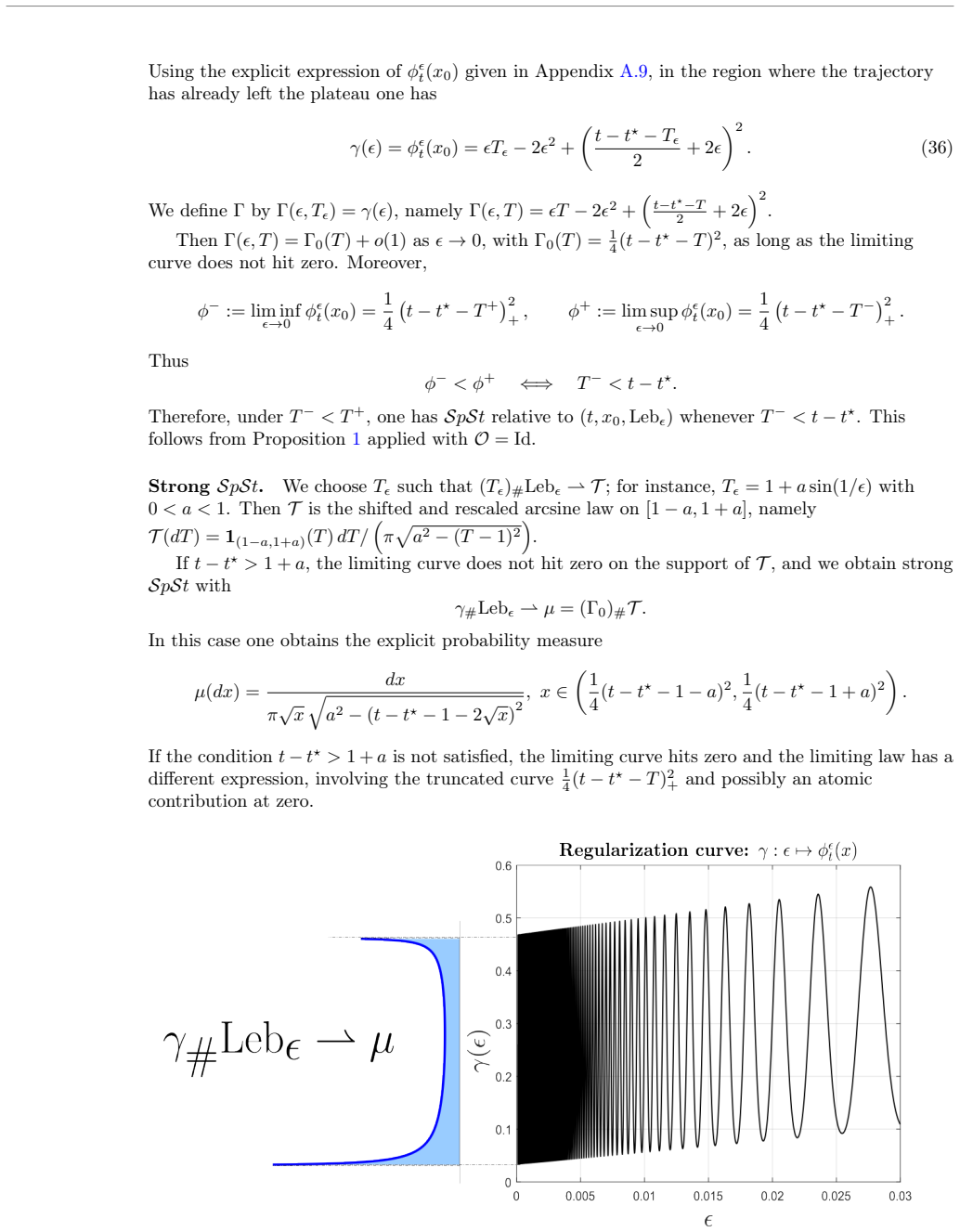
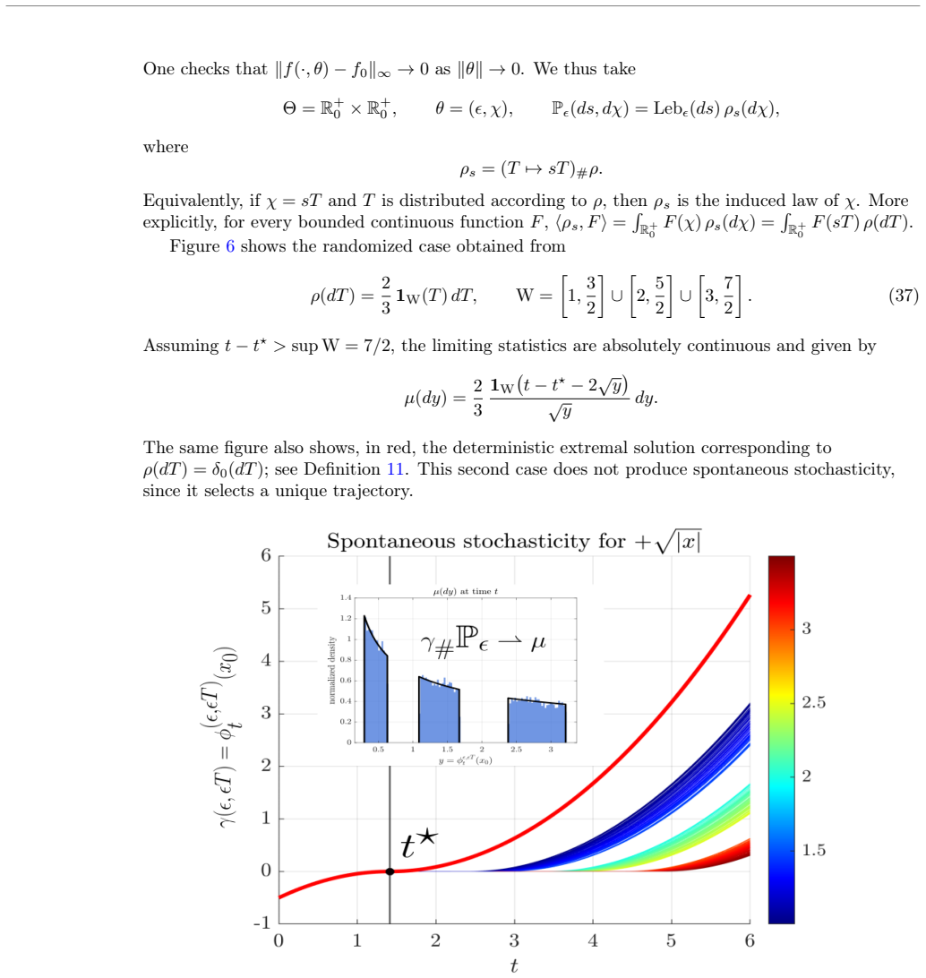
Summary. The paper proposes a measure-theoretic definition of spontaneous stochasticity (SpSt) as a selection principle: for a regularized ill-posed inviscid problem and an ambient sampling measure, one studies the pushforward of the ambient measure under the regularized flow, with strong SpSt meaning convergence to a unique non-Dirac law. The central claim is an attainability theorem (Theorem 1, §4.1): if the inviscid problem is nonunique, then every probability measure supported on the compact inviscid endpoint set is attainable as the unique limiting law of some admissible regularization, so that M = M₀ = P(S₀), and Corollary 3 concludes that every non-Dirac law can be realized by a strong-SpSt regularization. The paper also derives a Dini-type necessary condition for nonuniqueness (§5), analyzes the relation to TBM and sensitivity-to-initial-data criteria (§3), and develops a semigroup/RG viewpoint (§§7–10) in which limiting statistics appear as statistical attractors. Explicit one-dimensional examples, including the √|x| family with an arcsine-type waiting-time law and an exit-time analysis for x^{1/3}, are worked out in detail, together with numerics in appendices.
Significance. If Theorem 1 and its proof are correct, the paper delivers a striking structural result: once nonuniqueness is present, essentially arbitrary inviscid statistics are realizable by suitable regularizations, shifting the physical content of SpSt onto the choice of regularization class and ambient measure. The paper is also valuable for its explicit, parameter-free computations in Section 6 and Appendix B, its careful comparison of SpSt, SpSt_turb, and TBM, and its semigroup/RG reformulation of limiting statistics as statistical attractors. The explicit examples and the detailed exit-time analysis in Section 9 are concrete and reproducible. However, the central attainability theorem has two load-bearing gaps in its proof — the admissibility of the tube-field construction and the unproved switching endpoint estimate — so the significance is conditional on those being repaired.
major comments (2)
- [Section 4.1, Step 4 (tube-field construction)] The field f(·,τ) = θ_τ F_τ + (1−θ_τ) f₀ is claimed to lie in V₀ as defined in Eq. (1). But θ_τ vanishes outside a tubular neighborhood of the selected inviscid trajectory, so f(·,τ) equals f₀ outside that neighborhood. For a non-Lipschitz f₀ — precisely the case in which nonuniqueness occurs — f(·,τ) is not globally Lipschitz and hence is not an admissible regularization in V₀. Even if the solution from x₀ is unique because it stays in the tube, the proof does not establish γ_x ∈ Γ, so E ⊂ M is not proven. The construction must be amended to use a global Lipschitz approximation of f₀ compatible with the tube, or the admissibility class must be revised with a proof that the regularized flow is single-valued for the relevant initial data.
- [Section 4.1, Step 5, Eq. (24)] The pivotal assertion γ_θ(s) − γ̂_θ(s) = o(1) is stated without proof. It is not a routine continuity consequence: uniform convergence of f_θ(·,s) to f₀ does not imply convergence of finite-time flow maps when the limit field is non-Lipschitz (e.g., √x + η abandons the 'stay at zero' solution for arbitrarily small η). The coefficient a_θ(s) switches between the two tube fields on a fast scale, and the physical-time endpoint can depend on the entire switching history. Since this step is the only argument for co(E) ⊂ M, Theorem 1 and Corollary 3 collapse if it fails. The explicit examples in Section 6 do not exercise the switching construction, so they provide no corroboration. A proof, or a modified construction with quantitative estimates on the switching error, is required.
minor comments (5)
- [Corollary 3, Section 4.1] The statement 'M₀ \ E = M' contradicts the already-proved identity M = M₀; it should presumably read 'M₀ \ E = M \ E' or similar. Please correct this typographical-formulaic inconsistency.
- [Section 3.2.2, Property 1] Property 1 is asserted 'without proof'. As written, the implication TBM ⇒ liminf Var(ν_ε) ≥ L does not follow from Eq. (16), because the liminf of Var(κ_ε) at the endpoint does not control the Cesàro average of s ↦ Var(κ_s). Either add a hypothesis (e.g., continuity or a uniform lower bound on s ↦ Var(κ_s)) or downgrade the statement to a conjecture.
- [Section 6.2, Strong SpSt] The notation T_ε is used both for the regularization parameter value and for the function s ↦ T_s entering the curve γ(s). This creates the appearance that (T_ε)#Leb^ε is a Dirac mass. Please make explicit that T_ε denotes the function T(s) and write T_s or T(·) in the pushforward statement.
- [Appendix A.7, proof of Theorem 2] The Osgood argument should state explicitly that the modulus Ω is nondecreasing (or assume the appropriate Osgood condition on a nondecreasing function); otherwise the standard one-sided Osgood lemma does not directly apply to an arbitrary Ω with divergent integral.
- [General] Some displayed identities in Section 4.1 could benefit from numbering (e.g., the tube-field definition in Step 4 and the switching field in Step 5), since the current text refers to 'the previous construction' without precise equation numbers.
Circularity Check
No significant circularity; the central attainability theorem is constructive and self-contained.
full rationale
The paper's core derivation chain (Theorem 1 and Corollary 3, Section 4.1) does not reduce to its inputs by construction or by self-citation. M0 is defined independently as the simplex of probability measures on the inviscid endpoint set S0, and the nontrivial inclusion M0 ⊆ M is attacked by explicit constructions: Step 4 builds vector fields realizing each endpoint, Step 5 mixes curves for convex combinations, and Step 6 glues the approximating curves. The selected measure is the output of an explicit construction, not a fitted parameter or a renamed input. The explicit limiting laws in Section 6 and Appendix B are parameter-free computations once the stated regularizations are fixed, and the Section 9 exit-time analysis is again a direct calculation. The reviewer's main caveat is the unproved o(1) endpoint estimate in Step 5 of Theorem 1; near non-Lipschitz singularities, sup-norm field convergence does not automatically imply endpoint convergence for rapidly switching fields. That is a genuine proof gap and a correctness risk, but it is not circularity: the estimate is not assumed as the theorem's conclusion, and no equation identifies the target measure with a construction input. The self-citations in the paper, including the companion PDE paper [17] and the numerical study [32], appear in the perspective/discussion sections and are not load-bearing for the finite-dimensional attainability theorem. The finite-dimensional theorems are proved in the text, so the paper is self-contained with respect to its main claims.
Assumptions & free parameters
free parameters (6)
- Ambient measure family P^ε (convention P^ε = Leb^ε) =
Leb^ε = normalized Lebesgue on [0,ε] (other choices explored in Remark 2.3)
- Admissible regularization class V0 =
n/a — definitional
- Waiting-time shape T_ε in example (AmbTε) =
T_ε = 1 + a sin(1/ε), a ∈ (0,1); or 1 + a sin(b log ε)
- Switching-phase parameter c_θ in Theorem 1, Step 5 =
c_θ = sin(π(θ − 1/2))
- Modulus Ω in Theorem 2 =
unspecified ('one can find some Ω')
- RG generator G in Section 9 example =
G(Y) = χ − Y, χ ∈ S0; generalized to n equilibria
assumptions (7)
- standard math Peano existence theorem (f0 ∈ Cb ⇒ local existence for (P0))
- standard math Kneser's theorem: in finite dimension, S0 is compact and connected
- standard math Prokhorov, Krein-Milman, Arzelà-Ascoli, Stone-Weierstrass, dominated convergence
- domain assumption One-sided Osgood uniqueness lemma
- domain assumption Finite-dimensional compactness setting
- ad hoc to paper Existence of tube vector fields in V0 approximating arbitrary inviscid trajectories
- ad hoc to paper Ambient measure convention P^ε = Leb^ε (post-Remark 2.4)
Cite this review
Pith. "Pith review of A Measure-Theoretic Approach to Spontaneous Stochasticity." pith.science (2026). https://pith.science/paper/TJNXIRGK
@misc{pith2026260716328,
  author       = {Pith},
  title        = {Pith review of: A Measure-Theoretic Approach to Spontaneous Stochasticity},
  year         = {2026},
  howpublished = {\url{https://pith.science/paper/TJNXIRGK}},
  note         = {Machine review of arXiv:2607.16328}
}
read the original abstract
Spontaneous stochasticity (SpSt), originating in Richardson's picture of turbulent dispersion and Lorenz's Eulerian view of finite-time loss of predictability, was later formulated under this name by Gaw\k{e}dzki and collaborators and developed in shell models by Mailybaev and collaborators. Whether it occurs in fully developed turbulence remains a major open question. Beyond a few specific classes of systems, however, SpSt has lacked a general mathematical definition. We introduce a measure-theoretic formalism in which it is understood as a measure-selection principle. Given an inviscid problem, a well-posed regularization, and an ambient measure, we study the pushforward of that measure by the regularized flow. Strong SpSt occurs when these pushforward measures converge to a non-Dirac probability law, replacing classical deterministic selection by statistical selection. For finite-dimensional systems, we establish several structural results. Our central attainability theorem shows that, whenever the inviscid problem is nonunique, any probability measure supported on the set of inviscid states can be selected as the limiting law of a suitable regularization. We also identify singular sets in the inviscid dynamics, detected through Dini-type directional growth, as necessary obstructions underlying nonuniqueness. We analyze the relation between SpSt and sensitivity to initial data, clarifying the scope and limitations of turbulence-inspired finite-time separation criteria. Finally, we develop a renormalization-(semi)group viewpoint in which limiting statistics arise as statistical attractors. Explicit examples illustrate how ambient measures, inviscid singularities, regularization scales, and initial-data sensitivity interact in the emergence of SpSt.
Figures


Figures from the paper (8 more)



Forward citations
Cited by 1 Pith paper
-
Spontaneous stochasticity and anomalous dissipation in collapsing wave turbulence
A collapsing one-dimensional wave model is shown (numerically) to become spontaneously stochastic after blowup: vanishing regularization or initial-data perturbations produce finite post-blowup uncertainty.
Reference graph
Works this paper leans on
-
[1]
Series A, Containing Papers of a Mathematical and Physical Character110709–737
Richardson L 1926Proceedings of the Royal Society of London. Series A, Containing Papers of a Mathematical and Physical Character110709–737
-
[2]
Bernard D, Gaw¸ edzki K and Kupiainen A 1998J. Stat. Phys.90519–569
-
[3]
Chaves M, Gawedzki K, Horvai P, Kupiainen A and Vergassola M 2003J. Stat. Phys.113 643–692
-
[4]
Fluid Mech.829153–189
Drivas T and Eyink G 2017J. Fluid Mech.829153–189
-
[5]
Lorenz E 1969Tellus21289–307
-
[6]
Lorenz E 1963J. Atmos. Sci.20130–141
-
[7]
Eyink G and Bandak D 2020Phys. Rev. Res.2(4) 043161
-
[8]
Mailybaev A 2012Physical Review E85066317
Show all 35 references
-
[9]
Mailybaev A 2016Multiscale Modeling & Simulation1496–112
-
[10]
Mailybaev A and Raibekas A 2023Commun. Math. Phys.4012643–2671
-
[11]
Mailybaev A and Raibekas A 2023Arnold Math J.9339–357
-
[12]
Mailybaev A A 2025Nonlinearity38085010
-
[13]
Drivas T and Mailybaev A 2021Nonlinearity342296
-
[14]
Drivas T, Mailybaev A and Raibekas A 2024Ergodic Theo. and Dyn. Syst.441856–1884
-
[15]
Gradinaru M, Herrmann S and Roynette B 2001Annales de l’Institut Henri Poincaré Probabilités et Statistiques37555–580 ISSN 0246-0203
-
[16]
Mailybaev A A 2026Phys. Rev. Fluids11(3) 034605 39
-
[17]
Ruffenach W, Simonnet E and Valade N 2025 Spontaneous stochasticity in the Armstrong–Vicol passive scalar (Preprint2509.15683)
2025
-
[18]
Mailybaev A A 2025J. Stat. Phys.19237
-
[19]
Thalabard S, Bec J and Mailybaev A 2020Commun. Phys.3
-
[20]
Walter W 1970Differential and Integral Inequalities(Ergebnisse der Mathematik und ihrer Grenzgebietevol 55) (Springer)
-
[21]
Agarwal R and Lakshmikantham V 1993Uniqueness and Nonuniqueness Criteria for Ordinary Differential Equations(Series in Real Analysisvol 6) (Singapore: World Scientific) ISBN 978-981-02-1357-2
-
[22]
Hartman P 2002Ordinary Differential Equations2nd ed (Classics in Applied Mathematics vol 38) (SIAM) ISBN 978-0-89871-510-1
-
[23]
Bahouri H, Chemin J Y and Danchin R 2011Fourier Analysis and Nonlinear Partial Differential Equations(Grundlehren der mathematischen Wissenschaftenvol 343) (Springer)
-
[24]
Ambrosio L 2004Inventiones mathematicae158227–260
-
[25]
Flandoli F 2009Metrika69101–123
-
[26]
Mailybaev A A and Moriconi L 2026arXiv preprint(Preprint2602.24221)
-
[27]
Karabacak O and Ashwin P 2011Mathematical Proceedings of the Cambridge Philosophical Society150353–365
-
[28]
Arnold V I, Afrajmovich V S, Il’yashenko Y S and Shil’nikov L P 1999Bifurcation Theory and Catastrophe Theory(Encyclopaedia of Mathematical Sciencesvol 5) (Berlin, Heidelberg: Springer-Verlag) ISBN 978-3-540-65379-0
-
[29]
Feigenbaum M 1976Los Alamos Theoretical Division Annual Report98–102
-
[30]
Lasota A and Mackey M 1994Chaos, Fractals, and Noise: Stochastic Aspects of Dynamics 2nd ed (Applied Mathematical Sciencesvol 97) (Springer)
-
[31]
Armstrong S and Vicol V 2025arXiv preprint arXiv:2503.11744(Preprint2503.11744)
-
[32]
Ruffenach W 2026arXiv preprint
-
[33]
Giorgi G and Komlósi S 1992Rivista di matematica per le scienze economiche e sociali15 3–30
-
[34]
Bruckner A 1978Differentiation of Real Functions(Lecture Notes in Mathematicsvol 659) (Springer Berlin, Heidelberg) ISBN 978-3-540-08910-0
-
[35]
Osgood framework
Dombre T and Gilson J L 1998Physica D: Nonlinear Phenomena111265–287 A Appendix A.1 Equivalence of Definitions: Proposition 1 We justify Proposition 1. Figure 1 illustrates the mutually exclusive scenarios. In the definition of weakSpSt, it is not necessary to specify whether ...
Reviewed August 2, 2026 · model on record in the stance chip above.
Discussion (0). Continue with ORCID to comment.