REVIEW 3 major objections 4 minor 1 cited by
The Inflaton Effective Potential for General $\epsilon$
T0 review · 3 major / 4 minor · reviewed 2026-08-14 · deepseek-v4-flash
Pith's one-line read One-loop quantum corrections to the inflaton potential in a general slow-roll universe split into a local piece fixed by instantaneous $H$ and $\epsilon$ and a nonlocal piece fixed by past geometry, so no local counterterm in $\phi$ and…
desk verdict Local part is a real step beyond de Sitter, but the nonlocal tail is off by hundreds: Eq. (55) uses the massless frozen amplitude where the massive mode is still ~e^6 below it. read the letter →
The pith
A machine-rendered reading of the paper's core claim, the machinery that carries it, and where it could break.
The reading
What carries the argument
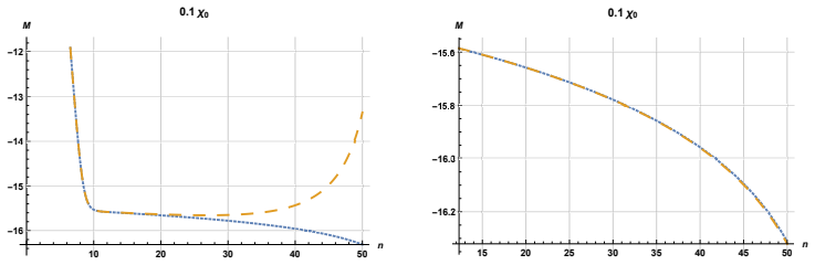
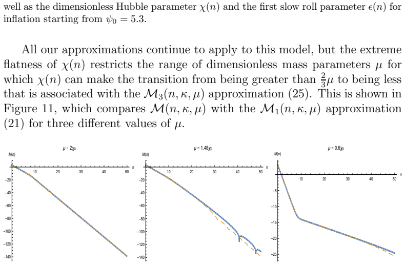
The central object is the three-phase analytic approximation to $M(n,\kappa,\mu) = \ln(|u(t,k,M)|^2\sqrt{8\pi G})$, the logarithm of the norm-squared of the scalar mode function, evolved in e-folding time $n$. The machinery is a matched sequence of approximations: $M_1$, the ultraviolet form written as a Hankel function of the first kind with slowly varying argument and index; $M_2$, the steady-decline form written with $\tanh$ of an integrated frequency $\omega$; and $M_3$, the oscillatory-decline form written with $\tan$ of an integrated frequency $\Omega$, joined at $n_\kappa+4$ and $n_\mu+4$. This decomposition isolates the ultraviolet divergences in $M_1$, allows the infrared contribution to factor into a wave-number part inherited from $M_1$ plus geometric functions $f_{2,3}$ that carry the memory of the past, and yields the nonlocal integral (56). The same vary-then-specialize procedure, together with stress-energy conservation, produces the modified Friedmann equations for a Lagrangian $a^3 f(H,\epsilon)$.
What would settle it
Solve the mode equation (16) numerically for a slow-roll model not used in the calibration, for instance a linear inflaton potential, over the same range of wave numbers and masses, and compare the exact coincidence limit with the sum of (53) and (59). If the difference is not within the claimed approximation, or if direct evaluation of the exponentials in (57)-(58) shows they are not small, the decomposition fails. A more targeted check is to evaluate the integral (56) exactly for a plateau potential and see whether it reproduces the simple negative integral (59).
Extended reading notes
Core claim
The paper establishes a decomposition of the one-loop inflaton effective potential for general slow-roll FRW backgrounds. Working with the logarithm $M(n,\kappa,\mu)$ of the norm-squared of the mode function of a minimally coupled scalar, it shows that $M$ is well described by three consecutive approximations: an ultraviolet form involving a Hankel function with slowly varying argument and index, a steady-decline form involving $\tanh$ of an integrated frequency, and an oscillatory-decline form involving $\tan$ of an integrated frequency, with transitions at about four e-foldings after horizon crossing and four e-foldings after mass domination. After renormalization with the conformal and quartic counterterms, the resulting effective potential consists of a local piece, expression (53), depending on instantaneous $H$, $\epsilon$, and $z = h^2\phi^2/(2H^2)$, plus a nonlocal piece, expression (59), equal to $(1/4)h^2\phi^2$ times a negative integral over past e-foldings of $(1-\epsilon)H^2$. Because the local piece is not a function of $R = 6(2-\epsilon)H^2$ alone and the nonlocal piece cannot be reproduced by any local action, no subtraction that is local in $\phi$ and $R$ can completely remove the correction.
Load-bearing premise
The result assumes that the mode amplitude always moves through the same three stages, ultraviolet, steady decline, and oscillatory decline, with the switch points at four e-foldings after horizon crossing and four e-foldings after mass domination, and that the leftover exponential factors in the nonlocal part are negligibly small.
Editorial extensions
If this is right
- The one-loop potential is not a function of $\phi$ and $R$ alone, so the two previously considered subtraction schemes (a function of the inflaton only, or a function of the inflaton and the Ricci scalar) cannot remove the correction.
- The nonlocal piece is a negative contribution to the inflaton mass-squared; for the quadratic model it subtracts roughly $75h^2/(16\pi^2)$ of the inflaton mass, which can be absorbed by changing the bare mass but not by a local counterterm.
- Because the correction is not suppressed by the gravitational scale, the paper concludes that unless the coupling $h$ is very small, the modified Friedmann equations change the background enough to make viable classical inflation difficult, and that cancellation between bosonic and fermionic contributions is a more promising route.
- The generalized Friedmann equations (64) and (62) reduce to the standard $F(R)$ equations when $f$ is restricted to the Ricci scalar, and to the earlier no-$\epsilon$-dependence result when $f$ is independent of $\epsilon$.
- The three-phase approximation also applies to plateau-type potentials, with the mass-domination phase occurring for only a narrow range of mass parameters.
Reading between the lines
- Editorial inference: the claim that the approximation is independent of the classical potential predicts that the same three-phase rule will hold for other slow-roll models, such as linear or natural inflation; checking the transition times there would be a direct test of universality.
- Editorial inference: the nonlocal memory term, if small but nonzero, implies that primordial perturbation observables like the spectral index and tensor-to-scalar ratio could be altered not only through the background $H$ and $\epsilon$ but also through changes to the linearized perturbation equations, a computation the paper leaves open.
- Editorial inference: the modified Friedmann equations contain higher time derivatives, and although the paper argues quantum corrections should be treated as perturbations rather than new degrees of freedom, a systematic derivation of the back-reaction equations for the nonlocal term (59) would be the next step toward quantitative predictions.
- Editorial inference: the negative mass-squared from the nonlocal piece might be combined with positive contributions from bosonic couplings to design models where the total correction is small; the paper mentions this possibility but offers no concrete model.
Editorial analysis
A structured set of objections, weighed in public.
Referee Report
Summary. The paper develops an analytic approximation for the logarithm of the norm-squared mode function of a massive, minimally coupled scalar in a spatially flat FRW background, organized into three phases: ultraviolet, steady decline, and oscillatory decline. It uses this approximation to compute the one-loop Coleman-Weinberg correction to the inflaton effective potential from the coupling (6). The claimed result consists of a local part (53) depending on the instantaneous Hubble parameter and slow-roll parameter, plus a nonlocal part (59) obtained from the infrared integral (56), with the nonlocal part argued to be small. The paper also derives modified Friedmann equations (64) and (62) for Lagrangians depending locally on H and epsilon, and it checks the mode-function approximations numerically for the quadratic and Starobinsky potentials.
Significance. If the central result holds, this paper would close a known gap in earlier de Sitter-based studies by showing explicitly how the one-loop inflaton effective potential depends on a general slow-roll geometry, and it would strengthen the argument that local counterterms involving only the inflaton and the Ricci scalar cannot fully remove the correction. The paper contains genuine analytic derivations in Section 2.3, numerical validation of the phase approximations for two inflaton potentials, recovery of the flat-space Coleman-Weinberg limit, and consistent F(R) limits for the generalized Friedmann equations. However, the quantitative nonlocal formula (59) is not yet supported because of the prefactor issue identified below, so the present version cannot be accepted as a finished calculation of the nonlocal part.
major comments (3)
- [Section 3, Eqs. (54)-(55)] The step from (54) to (55) replaces the massive amplitude e^{M1(n_kappa+4, kappa, mu)} by the massless frozen value H^2(t_kappa)/(2 sqrt(8 pi G) k^3). This omits the massive post-horizon suppression. For the paper's own mu = 1.2 chi_0 case, with n_kappa = 8.32 and n_2 = 12.32, the small-z evaluation of (21) gives nu approximately 0.6, so e^{M1(n_2)} is approximately e^{-5.5} H^2(t_kappa)/(2 sqrt(8 pi G) k^3). The replacement therefore overstates the infrared integrand by a factor of order e^{5.5} approximately 250 for these modes, and by more for earlier-crossing modes. Because this replacement feeds directly into (56) and hence into (59), the quantitative nonlocal result and the associated claim that the nonlocal part is small are not controlled by the mode-function approximations derived in the paper. The local part (53) and the generalized Friedmann equations (62) and (64) are not affected by this issue.
- [Section 2.2 and Section 3, transition times n_2 and n_3] The choice of transition times n_2 = n_kappa + 4 and n_3 = n_mu + 4 is calibrated by visual inspection of numerical plots for the quadratic potential, and no sensitivity study or error estimate is provided. The prefactor e^{M1(n_2)} in (54) and the nonlocal exponentials (57)-(58) depend on these offsets, so the extension of the approximation to arbitrary slow-roll backgrounds is not established by the two tested models. A derivation of the offset, or at least a quantitative bound on the error it induces, is needed to support the general-epsilon claim.
- [Section 3, Eq. (59)] The reduction of the nonlocal part to the simple expression (59) is made under the stated 'expected' assumption that the factors in (57)-(58) are small, but no estimate, bound, or numerical check of this smallness is supplied. Given the prefactor problem in the transition from (54) to (55), the smallness of the nonlocal contribution needs independent verification before (59) can be used as a quantitative result.
minor comments (4)
- [Abstract and Epilogue] There are typos: 'mass ive scalar' in the abstract and 'Coelman-Weinberg' in the Epilogue; these should be corrected.
- [Section 2.2, Figure captions] The text states that Delta M(n, mu) rapidly freezes to a constant after horizon crossing, but the middle and right panels of Figure 8 and all of Figure 9 show non-constant or oscillatory late-time behavior; the captions or the surrounding discussion should be clarified to distinguish the regimes in which the freezing claim holds.
- [Section 3, Eq. (43)] The transition wave number K(n) is defined by K(n) = e^{n-4} chi(n-4) sqrt(8 pi G), which amounts to exactly four e-foldings after horizon crossing; this is a natural definition, but the paper should state explicitly that the factor of four is the same visually calibrated offset used elsewhere, and should note the residual uncertainty from that calibration.
- [Section 4] The statement that F(R) models are the unique local and invariant modification of general relativity avoiding kinetic instabilities should be attributed more carefully to the cited review [12], since it depends on specific assumptions about the Lagrangian class considered.
Circularity Check
The effective-potential calculation is self-contained: the mode-function approximations are derived analytically and checked against numerical integration, and prior self-citations are motivational rather than load-bearing.
full rationale
The derivation of the one-loop inflaton effective potential is not circular. The mode-function amplitude M(n,κ,μ) is obtained from the nonlinear equation (16) with WKB initial conditions (18), and the three phase approximations M1, M2, and M3 are validated against direct numerical integration in Figures 1-9. The M1 form is also given an independent analytic derivation in Section 2.3 through the expansion in equations (30)-(32). The local part (53) and the nonlocal part (56)-(59) are then computed from these approximations by explicit integration and dimensional regularization, and the flat-space Coleman-Weinberg limit is recovered as a check. Prior self-cited work enters only as motivation, such as the de Sitter result [9] and the Hubble-effective-potential motivation [16], or as context for applications in [10]-[12]; none of these citations supplies the central computational input. The conclusion that no local counterterm depending only on φ and R can remove the correction follows from the explicit factors of H and ε visible in (53), combined with the standard external uniqueness statement [12], rather than from a fitted parameter being renamed as a prediction. The skeptical concern that equation (55) overstates the infrared integrand is a numerical-accuracy critique of an approximation, not a demonstration that the result is equivalent by construction to its input. The paper also explicitly flags the smallness assumption needed for equation (59), which is an assumption rather than a circular step. No circular step can be exhibited.
Assumptions & free parameters
free parameters (1)
- phase transition offset Δn =
4 e-foldings
assumptions (5)
- domain assumption The background geometry is a spatially flat FRW metric with slowly varying H and ε such that the slow-roll expressions (14) are accurate and the WKB initial conditions (17-18) apply at the start of inflation.
- domain assumption The phase-transition offsets n2 = nκ + 4 and n3 = nµ + 4 are universal for arbitrary slow-roll models, not only the quadratic and Starobinsky potentials tested numerically.
- domain assumption The exponentials of f2(n,µ) and f3(n,µ) in (57-58) are small enough that expanding them to leading order gives the nonlocal result (59).
- standard math Palais's theorem and stress-energy conservation allow reconstructing the g00 Friedmann equation from the gij equation for an action specialized to FRW.
- standard math Dimensional regularization and the standard scalar mode-function Wronskian normalization (9) govern the ultraviolet computation.
Cite this review
Pith. "Pith review of The Inflaton Effective Potential for General $\epsilon$." pith.science (2026). https://pith.science/paper/TKO6FE4Y
@misc{pith2026190803814,
  author       = {Pith},
  title        = {Pith review of: The Inflaton Effective Potential for General $\epsilon$},
  year         = {2026},
  howpublished = {\url{https://pith.science/paper/TKO6FE4Y}},
  note         = {Machine review of arXiv:1908.03814}
}
read the original abstract
We develop an analytic approximation for the coincidence limit of a massive scalar propagator in an arbitrary spatially flat, homogeneous and isotropic geometry. We employ this to compute the one loop corrections to the inflaton effective potential from a quadratic coupling to a minimally coupled scalar. We also extend the Friedmann equations to cover potentials that depend locally on the Hubble parameter and the first slow roll parameter.
Figures


Figures from the paper (8 more)




Forward citations
Cited by 1 Pith paper
-
Ricci Subtraction for Cosmological Coleman-Weinberg Potentials
Ricci-scalar subtraction of cosmological Coleman-Weinberg potentials introduces a higher-derivative degree of freedom that ends inflation within roughly one e-folding.
Reference graph
Works this paper leans on
- [1]
- [2]
-
[3]
A. H. Guth, D. I. Kaiser and Y. Nomura, Phys. Lett. B 733, 112 (2014) doi:10.1016/j.physletb.2014.03.020 [arXiv:1312.7619 [astro-ph.CO]]
arXiv 2014
-
[4]
Linde, doi:10.1093/acprof:oso/9780198728856.003.0006 arXiv:1402.0526 [hep-th]
A. Linde, doi:10.1093/acprof:oso/9780198728856.003.0006 arXiv:1402.0526 [hep-th]
-
[5]
A. H. Guth et al. [33 co-authors], “A Cosmic Controversy,” (Letter to the Editor), Scientific American (May 10, 2017)
work page 2017
- [6]
-
[7]
S. R. Coleman and E. J. Weinberg, Phys. Rev. D 7, 1888 (1973). doi:10.1103/PhysRevD.7.1888
-
[8]
D. R. Green, Phys. Rev. D 76, 103504 (2007) doi:10.1103/PhysRevD.76.103504 [arXiv:0707.3832 [hep-th]]. 24
arXiv 2007
Show all 33 references
-
[9]
S. P. Miao and R. P. Woodard, JCAP 1509, no. 09, 022 (2015) doi:10.1088/1475-7516/2015/09/022, 10.1088/1475-7516/201 5/9/022 [arXiv:1506.07306 [astro-ph.CO]]
2015 arXiv
-
[10]
J. H. Liao, S. P. Miao and R. P. Woodard, Phys. Rev. D 99, no. 10, 103522 (2019) doi:10.1103/PhysRevD.99.103522 [arXiv:1806.02533 [g r- qc]]
2019 arXiv
-
[11]
S. P. Miao, S. Park and R. P. Woodard, Phys. Rev. D 100, no.10, 103503 (2019) doi:10.1103/PhysRevD.100.103503 [arXiv:1908.05558 [gr-qc]]
2019 arXiv
-
[12]
R. P. Woodard, Lect. Notes Phys. 720, 403 (2007) doi:10.1007/978-3- 540-71013-4 14 [astro-ph/0601672]
2007 arXiv
-
[13]
Finelli, G
F. Finelli, G. Marozzi, A. A. Starobinsky, G. P. Vacca and G. Ven- turi, Phys. Rev. D 79, 044007 (2009) doi:10.1103/PhysRevD.79.044007 [arXiv:0808.1786 [hep-th]]
2009 arXiv
-
[14]
M. G. Romania, N. C. Tsamis and R. P. Woodard, JCAP 1208, 029 (2012) doi:10.1088/1475-7516/2012/08/029 [arXiv:1207.3227 [astro- ph.CO]]
2012 arXiv
-
[15]
D. J. Brooker, N. C. Tsamis and R. P. Woodard, Phys. Rev. D 93, no. 4, 043503 (2016) doi:10.1103/PhysRevD.93.043503 [arXiv:1507.0745 2 [astro-ph.CO]]
2016
-
[16]
T. M. Janssen, S. P. Miao, T. Prokopec and R. P. Woodard, JCA P 0905, 003 (2009) doi:10.1088/1475-7516/2009/05/003 [arXiv:0904.115 1 [gr-qc]]
2009 doi
-
[17]
I. S. Gradshteyn and I. M. Ryzhik, Table of Integrals, Series a nd Prod- ucts, 4th Edition, (New York, Academic Press, 1965)
1965
-
[18]
R. S. Palais, Commun. Math. Phys. 69, no. 1, 19 (1979). doi:10.1007/BF01941322
1979 doi
-
[19]
J. Z. Simon, Phys. Rev. D 41, 3720 (1990). doi:10.1103/PhysRevD.41.3720
1990 doi
-
[20]
A. A. Starobinsky, Adv. Ser. Astrophys. Cosmol. 3, 130-133 (1987) doi:10.1016/0370-2693(80)90670-X 25
1987 doi
-
[21]
D. J. Brooker, S. D. Odintsov and R. P. Woodard, Nucl. Phys. B 911, 318-337 (2016) doi:10.1016/j.nuclphysb.2016.08.010 [arXiv:1606.058 79 [gr-qc]]
2016 doi
-
[22]
Candelas and D
P. Candelas and D. J. Raine, Phys. Rev. D 12, 965 (1975). doi:10.1103/PhysRevD.12.965
1975 doi
-
[23]
S. P. Miao and R. P. Woodard, Phys. Rev. D 74, 044019 (2006) doi:10.1103/PhysRevD.74.044019 [gr-qc/0602110]
2006 arXiv
- [24]
-
[25]
Prokopec, N
T. Prokopec, N. C. Tsamis and R. P. Woodard, Annals Phys. 323, 1324 (2008) doi:10.1016/j.aop.2007.08.008 [arXiv:0707.0847 [gr-qc]]
2008 arXiv
- [26]
-
[27]
D. J. Brooker, N. C. Tsamis and R. P. Woodard, Phys. Rev. D 96, no.10, 103531 (2017) doi:10.1103/PhysRevD.96.103531 [arXiv:1708.03253 [g r- qc]]
2017 arXiv
-
[28]
D. J. Brooker, N. C. Tsamis and R. P. Woodard, JCAP 04, 003 (2018) doi:10.1088/1475-7516/2018/04/003 [arXiv:1712.03462 [gr-qc]]
2018 arXiv
-
[29]
S. Basu, D. J. Brooker, N. C. Tsamis and R. P. Woodard, Phys. Rev. D 100, no.6, 063525 (2019) doi:10.1103/PhysRevD.100.063525 [arXiv:1905.12140 [gr-qc]]
2019 arXiv
-
[30]
S. P. Miao, L. Tan and R. P. Woodard, [arXiv:2003.03752 [gr-qc]]
2003 arXiv
-
[31]
E. O. Kahya and R. P. Woodard, Phys. Rev. D 76, 124005 (2007) doi:10.1103/PhysRevD.76.124005 [arXiv:0709.0536 [gr-qc]]
2007 arXiv
-
[32]
E. O. Kahya and R. P. Woodard, Phys. Rev. D 77, 084012 (2008) doi:10.1103/PhysRevD.77.084012 [arXiv:0710.5282 [gr-qc]]
2008 arXiv
-
[33]
N. C. Tsamis and R. P. Woodard, Phys. Rev. D 54, 2621 (1996) doi:10.1103/PhysRevD.54.2621 [hep-ph/9602317]. 26
1996 arXiv
Reviewed August 14, 2026 · model on record in the stance chip above.
Discussion (0). Continue with ORCID to comment.