Efficient Reduction of Interconnected Subsystem Models using Abstracted Environments

Bart Besselink; Luuk Poort; Nathan van de Wouw; Rob H.B. Fey

REVIEW 3 major objections 2 minor 27 references

Efficient Reduction of Interconnected Subsystem Models using Abstracted Environments

T0 review · 3 major / 2 minor · reviewed 2026-08-10 · deepseek-v4-flash

Challenge this review Re-run · record.json Download PDF Read on arXiv ↗ Review JSON

Pith's one-line read Per-subsystem H-infinity error bounds, fixed a priori, guarantee the reduced interconnected model is stable and accurate; the environment-abstraction variant cuts a wafer-stage model to 128 states where an existing method needs 156.

desk verdict Nice framework, but Theorem 1's error formula fails a zero-error sanity check, so the central guarantee is not supported as written. read the letter →

arxiv 2501.11406 v1 pith:TMWSOAUL submitted 2025-01-20 eess.SY cs.SY

Luuk Poort , Bart Besselink , Rob H.B. Fey , Nathan van de Wouw This is my paper · ORCID

classification eess.SYcs.SY MSC 93B1193A1593B3693C05

keywords modelorderreductioninterconnectedsystemsabstractedenvironmentstructure-preservingrobustperformanceanalysisH-infinityerrorboundsbalancedtruncationwaferstagebenchmark

verification ladder T0 review T1 audit T2 compute T3 formal

The pith

A machine-rendered reading of the paper's core claim, the machinery that carries it, and where it could break.

The reading

The paper extends structure-preserving model reduction from reducing one subsystem against the full system to reducing every subsystem of an interconnected system, each against a cheap low-order stand-in for its environment. The central claim is that a user-specified accuracy bound on the reduced interconnected model can be converted, a priori, into weighted H-infinity bounds on the abstraction and reduction errors of each individual step; any abstraction and reduction that meet those low-level bounds automatically yield a well-posed, internally stable reduced interconnection whose error satisfies the high-level bound. Two variants are analysed: abstracting each environment as a whole (RAR-E) and abstracting the other subsystems one by one and interconnecting the abstractions (RAR-Sigma). On a 300-state wafer-stage benchmark, RAR-E produces a 128-state interconnected model while the prior robust subsystem reduction method needs 156 states for equal-or-worse accuracy; RAR-Sigma reaches 178 states yet yields the most accurate reduced model.

What carries the argument

The load-bearing identity is Lemma 3, equation (16): $\hat{\Sigma}_B = F_u\left(\begin{bmatrix} -\breve{E}_{B,22} & I \\ I & 0 \end{bmatrix}, \Sigma_B(I - \breve{E}_{B,22}\Sigma_B)^{-1} + (G_y)^{-1}\Lambda_{F,22}(G_u)^{-1}\right)$, which states that the full diagonal of reduced subsystems is exactly reconstructible from the full-order subsystems, the $22$-blocks of the abstracted environments, and the $22$-partition reduction errors alone, with all other partitions dropping out of the expression. Theorems 1 and 2 then pull the abstraction errors out of the abstracted environment blocks to write $\Lambda_C$ as an upper LFT of the connection matrix $N_E$ (environment abstraction) or $N_\Sigma$ (subsystem abstraction) against a block-diagonal error operator in which each abstraction error appears in its $22$-block form, each reduction error appears weighted as $(G_y)^{-1}\Lambda_{F,22}(G_u)^{-1}$, and the whole loop closes around the interconnection $S$. Theorem 3 converts this structure into a sufficient condition of robust-performance type: a frequency-wise scaling inequality $(VNW)(i\omega) D_r (VNW)^H(i\omega) \preceq D_l$ with structured scaling pairs $(D_l, D_r)$ drawn from the sets $\mathbb{D}_E$ or $\mathbb{D}_\Sigma$, which are defined through permutation matrices that sort the error blocks and frequency-wise positive-definite Hermitian blocks. The user-supplied weighting matrices $V$, $W$ and the gains $G_u$, $G_y$ tune how accuracy is distributed among the $22$-blocks and the rest of each subsystem.

What would settle it

Construct a small interconnected system (two or three subsystems) and produce reduced subsystems that satisfy the computed weighted bounds on the 22-partition errors while deliberately making the non-22 partitions of the reduction and abstraction errors large, for instance by perturbing only those blocks. If the resulting interconnected error $\Lambda_C$ violates the prescribed specification even though the scaling inequality (42) holds with the claimed scalings, the 22-only sufficiency claim of Theorem 3 would be refuted; the same test would also expose whether Lemma 3's deferred proof, taken from reference [16], fails to cover the multi-subsystem case.

Watch

Extended reading notes

Core claim

The paper's central discovery is an exact error identity. The authors show that the diagonal of reduced subsystems $\hat{\Sigma}_B$ can be rewritten as an upper linear-fractional transformation whose perturbation depends on the unreduced subsystems, the $22$-blocks of the abstracted environments, and only the $22$-block partition of each subsystem's reduction error $\Lambda_F$ (Lemma 3). Pulling the abstraction errors out as well, the total interconnected error $\Lambda_C = F_l(S,\hat{\Sigma}_B) - F_l(S,\Sigma_B)$ becomes an upper LFT of a fixed connection matrix $N_E$ or $N_\Sigma$, built from the interconnection $S$, the unreduced subsystems, and the abstracted environment blocks, against a block-diagonal collection of the low-level abstraction errors $\Lambda_{E,22}$ or $\Lambda_A$ and weighted reduction errors $\tilde{\Lambda}_F$. This makes $\Lambda_C$ a structured feedback loop of small errors, so robust-performance theory applies: if each low-level error meets its weighted $\mathcal{H}_\infty$ bound and a scaling matrix pair $(D_l, D_r)$ satisfies $(VNW)(i\omega) D_r (VNW)^H(i\omega) \preceq D_l$ for all real $\omega$, then the reduced interconnection is stable and $\Lambda_C$ meets the prescribed weighted bound (Theorem 3). An accompanying optimization (Theorem 4) finds the most lenient low-level bounds that still guarantee the high-level specification, turning order selection from trial-and-error into a systematic procedure.

Load-bearing premise

The guarantee rests on the assertion, proved in the authors' earlier paper rather than here, that the reduced subsystems can be reconstructed from the unreduced subsystems, the abstracted-environment 22-blocks, and only the 22-partition reduction errors; the paper itself notes that the accuracy of other partitions also influences the overall error, so this 22-only sufficiency claim carries the whole result.

Editorial extensions

If this is right

Order selection becomes systematic: Algorithms 3 and 4 first solve the scaling optimization to obtain the most lenient low-level error bounds, then reduce each environment and subsystem to the lowest order meeting its bound, so no trial and error is needed.
The reduced model is still an interconnection of individually reduced subsystems, so the modular structure is preserved and each design team can keep its own subsystem model.
The expensive structure-preserving reduction is applied to each subsystem against an abstracted environment of much lower order than the full interconnection (in the benchmark, orders 26 to 116 instead of 200), which is what makes the method tractable for large assemblies.
On the wafer-stage benchmark, the environment-abstraction variant RAR-E attains a 128-state reduced interconnected model, 28 states smaller than the 156-state model of the existing robust subsystem reduction method, with equal or better accuracy; the subsystem-abstraction variant RAR-Sigma is the most accurate but the largest at 178 states.
Stability and the prescribed accuracy specification hold by construction: any abstraction and reduction meeting the computed low-level bounds yield a well-posed, internally stable reduced model with $\Lambda_C$ inside the prescribed set.

Reading between the lines

Editorial extensions of the paper, not claims the author makes directly.

Because the error identity only involves the $22$-partitions, the method's conservatism should grow with the strength of cross-coupling between subsystems; a sweep over coupling stiffness on the wafer-stage model would map where the abstraction step pays off and where the bounds become the bottleneck.
The paper's comparison implies that choosing the weighting functions $V$ and $W$ is the dominant source of conservatism; an automated, per-frequency weight design, of the kind the authors test in Section 6.3, would likely bring RAR-$\Sigma$'s required order close to RAR-$E$'s.
RAR-$\Sigma$'s modularity suits early design stages, where only rough subsystem models exist; using each newly computed reduced model as the abstraction for the next subsystem, which the paper notes is possible, should further reduce order and is a cheap iterative extension to test.
The a priori guarantee is only sufficient, not necessary; on systems where the $22$-block errors dominate, the reduced orders computed by Algorithms 3 and 4 may be far from the minimal orders that actually meet the specification, so a post-hoc check of the realized errors could unlock further reduction.

Share X Bluesky LinkedIn Reddit HN

Editorial analysis

A structured set of objections, weighed in public.

Desk editor's note, referee report, and a circularity audit.

Desk Editor's Note

read the letter

Luuk's paper has a good idea: reduce each subsystem against a low-order abstraction of its environment, then use robust-performance arguments to turn a high-level accuracy specification on the interconnection into low-level error bounds on the abstraction and reduction steps. That is a practical way to make structure-preserving reduction tractable, and the two variants (whole-environment and per-subsystem abstraction) cover the modularity/accuracy trade-off. The wafer-stage benchmark is also encouraging: RAR-E lands at 128 states versus 156 for the existing RSS method with comparable or better accuracy.

The problem is in the math that is supposed to make the guarantees formal. Theorem 1 gives an explicit LFT expression for the interconnected error Lambda_C in terms of abstraction and reduction errors. That expression fails the most basic consistency test. Take a single scalar subsystem, S = [0 1; 1 0], Sigma = 2, zero reduction error, and any nonzero abstraction error, say 0.1. If the reduction error is zero, the reduced subsystem is exactly Sigma, so the true interconnected error must be zero. The printed N_E, with M = 2 and Z = 0, gives F_u(N_E, diag(0.1, 0, 0.1)) = -0.2353. That is not zero. The formula is simply wrong as written, or at least incompatible with its own definitions. Since Theorem 3 and the optimization of Theorem 4 are built on this expression, the a-priori stability and accuracy guarantees are not established. The proof is 'omitted for brevity' and deferred to the authors' prior work [16], which is not adequate when the printed result fails a sanity check.

There are lesser issues too. Lemma 3 is also deferred to [16], and Section 5.3 concedes that non-22 partitions influence overall accuracy, so the sufficiency claim for 22-only bounds is non-obvious. The computational-cost advantage is asserted but not demonstrated; the benchmark shows RAR-E requiring more effort for the structure-preserving step. And there is a single example without code or data.

That said, the framework is clearly thought out, the writing is careful, and the idea is worth pursuing. This is not a circular argument or a fitted result; the error bounds are user-chosen weights, and the benchmark is legitimate. I would send this to a serious referee with a request to fix Theorem 1 and provide the full proof. As is, I would not cite the guarantee.

Referee Report

3 major / 2 minor

Summary. The paper proposes two structure-preserving model-reduction frameworks for interconnected linear time-invariant systems. In both frameworks, each subsystem is reduced while connected to a low-order abstraction of its environment, where the environment is abstracted either as a whole (Algorithm 1) or by abstracting the other subsystems individually (Algorithm 2). The authors use robust-performance analysis to translate a prescribed accuracy specification on the reduced interconnected system into sufficient low-level accuracy specifications on the abstraction and reduction errors. The main theoretical results are Theorem 1 and Theorem 2, which express the interconnected error as an upper LFT of the low-level errors, and Theorem 3, which gives a frequency-domain scaling condition guaranteeing stability and accuracy of the reduced interconnected model. The framework is demonstrated on a 2D wafer-stage structural-dynamics benchmark, where environment abstraction (RAR-E) achieves a 128-state reduced interconnected model compared with 156 states for robust subsystem reduction (RSS).

Significance. If the main theorems were correct, the paper would offer a useful modular reduction framework with a priori stability and accuracy guarantees and a systematic way to choose reduction orders. The connection between environment abstraction and robust performance is natural, and the benchmark is a relevant industrial example. The paper also deserves credit for providing explicit algorithms (Algorithms 1-4) and for attempting to quantify conservatism in Section 6.3. However, the central error expression in Theorem 1 fails a basic exact-reduction consistency test, and the proofs of Lemma 3 and Theorems 1 and 3 are either deferred or sketched. Since Theorem 3 and Theorem 4 inherit Theorem 1, the claimed guarantees are not established as written. The computational-efficiency claim is also not supported by the benchmark, which reports higher computational cost for the proposed methods.

major comments (3)

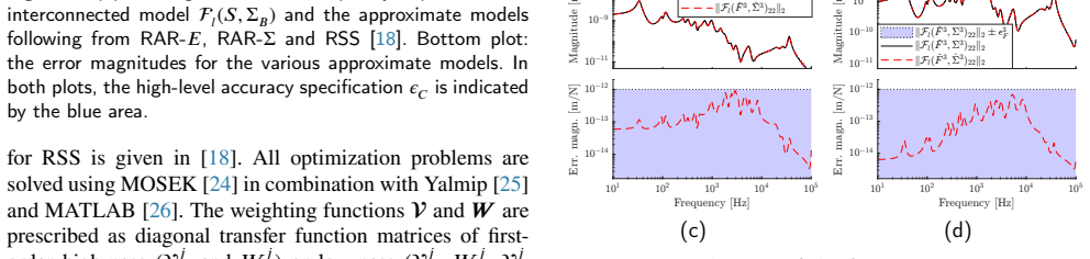
[Section 4.1.1, Eq. (22)] Theorem 1's expression for N_E is inconsistent with a simple exact-reduction test. Take k=1, S=[0 1; 1 0], Sigma=2, G_u=G_y=1, and abstracted environment block \check E_22=0.1. If the reduction error is zero (\tilde Lambda_F=0), then \hat Sigma=Sigma and the true interconnected error is Lambda_C=0 by definition (14). In (22)-(24), Z=S22-E_B,22=0 and M=(I-Sigma S22)^{-1} Sigma=2, so the right-hand side of (21) becomes F_u(N_E, diag(0.1,0,0.1)) = -0.2353, which is not 0. For a nonzero reduction error delta=0.01, direct evaluation gives Lambda_C=0.006395, while the printed formula gives -0.2303. Thus Eq. (22) is not a valid realization of the interconnected error dynamics. Since Theorem 3 and Theorem 4 both rely on this expression, the a-priori stability and accuracy guarantees are unsupported as stated. The authors must correct N_E and re-verify all downstream results.
[Section 4.1, Lemma 3 (Eq. (16))] Lemma 3 is load-bearing because Theorems 1 and 2 use it to express \hat Sigma_B in terms of only the 22-partition reduction errors. Its proof is deferred to the authors' preprint [16, Lemma 2], and the paper itself notes in Section 5.3 that 'the accuracy of other partitions also influences the overall accuracy' of the interconnected model. This creates an apparent contradiction between the claimed sufficiency of the 22-only error terms and the acknowledged influence of the other partitions. A complete proof of Lemma 3, or a clear explanation of why the other partitions can be neglected in the error bound, is required before Theorem 3 can be accepted.
[Section 6.2 and Abstract] The abstract and introduction claim that the approach 'significantly reduces the computational costs of reduction', but the benchmark shows the opposite for the considered example. The text after Table 2 states that RAR-E 'requires more computational resources for the structure-preserving reduction of F_l(\check F_j,Sigma_j) than RSS requires for the subsystem reduction of Sigma_j' and that RAR-Sigma is even more costly. The subsequent argument that costs would be similar for very high-order systems is speculative and not demonstrated by any complexity analysis or additional experiment. The efficiency claim should be either substantiated or substantially qualified.

minor comments (2)

[Section 6.2] There is a typo in the sentence 'RSS andand RAR-Sigma result in reduced models of higher order'; 'andand' should be 'and'.
[Section 5.1, Theorem 4] The notation 'given \check V, W' in (51) is ambiguous; Theorem 4 should specify whether the given weighting is \check V_E or \check V_Sigma, consistent with (44)-(45).

Circularity Check

0 steps flagged · score 0.0 of 10

No significant circularity: the error-propagation guarantees are sufficient-condition derivations, and the benchmark outcomes are not used as fitting targets.

full rationale

The derivation chain is not circular. The paper defines low-level errors in (11)-(14), rewrites the interconnected error as an upper LFT of abstraction and reduction errors in Theorems 1 and 2, and then gives a sufficient LMI condition in Theorem 3 under which weighted H-infinity bounds on those low-level errors imply the high-level accuracy specification. The low-level bounds are user-chosen or optimized variables, not parameters fitted to the benchmark outputs; the reduced orders and final errors are outcomes, not inputs to the method. The main debt to the authors' prior work [16] is for proof templates and prior lemmas, and the paper states the needed results explicitly rather than defining them in terms of the target claim. The omitted proof of Theorem 3 and the deferred proof of Lemma 3 are completeness or verification gaps, not logical circularity. Section 5.3's caveat that non-22 partitions also matter is an acknowledged limitation, not evidence that the guarantee reduces to its own assumptions. No step is shown to be equivalent to its inputs by construction.

Assumptions & free parameters 2 free parameters · 4 assumptions · 0 invented entities

The central claim rests on standard robust control machinery (scaled small-gain) plus the explicit well-posedness and stability Assumption 1. The user-chosen weighting functions and gain matrices are tuning knobs of the algorithm, not data-fitted constants, and no new physical entities are postulated. The main reliance on prior work is the deferred proof of Lemma 3, which is counted under soundness.

free parameters (2)

Weighting functions V and W = not reported numerically; user-selected first-order filters in benchmark
These define the error sets for abstraction, reduction, and interconnected accuracy. The paper notes in Sections 5.3 and 6.3 that their choice significantly affects conservatism and achievable reduction. They are hand-selected inputs, not fitted constants.
Gain matrices G_u and G_y = set to inverse weights as in Eq. (56) in benchmark
They trade reduction order against accuracy of the abstracted closed loop (Remark 1). The theory allows any nonsingular G_u and G_y, so the central claim does not depend on specific values.

assumptions (4)

domain assumption Assumption 1: all subsystems and the interconnection are internally stable and well-posed, and each environment E_j is stable.
Stated in Section 2.1; all LFTs and error models are defined on RH-infinity.
domain assumption Weighting functions V and W are bistable and biproper.
Required by Theorem 3 to guarantee stability; the paper notes the user can always choose them to satisfy this.
standard math Scaled small-gain / structured singular value upper bound provides a valid sufficient condition for robust stability and performance.
Invoked in Theorem 3 via the inequality S(i omega) D_r S^H(i omega) <= D_l for all omega; this is a standard robust control result.
standard math Block-diagonal LFTs commute (Lemma 2).
Used to collect environments and to express hat Sigma_B; proved in the text.

how reviews work

0 comments

Cite this review

Pith. "Pith review of Efficient Reduction of Interconnected Subsystem Models using Abstracted Environments." pith.science (2026). https://pith.science/paper/TMWSOAUL

@misc{pith2026250111406,
  author       = {Pith},
  title        = {Pith review of: Efficient Reduction of Interconnected Subsystem Models using Abstracted Environments},
  year         = {2026},
  howpublished = {\url{https://pith.science/paper/TMWSOAUL}},
  note         = {Machine review of arXiv:2501.11406}
}

read the original abstract

We present two frameworks for structure-preserving model order reduction of interconnected subsystems, improving tractability of the reduction methods while ensuring stability and accuracy bounds of the reduced interconnected model. Instead of reducing each subsystem independently, we take a low-order abstraction of its environment into account to better capture the dynamics relevant to the external input-output behaviour of the interconnected system, thereby increasing accuracy of the reduced interconnected model. This approach significantly reduces the computational costs of reduction by abstracting instead of fully retaining the environment. The two frameworks differ in how they generate these abstracted environments: one abstracts the environment as a whole, whereas the other abstracts each individual subsystem. By relating low-level errors introduced by reduction and abstraction to the resulting high-level error on the interconnected system, we are able to translate high-level accuracy requirements (on the reduced interconnected system) to low-level specifications (on abstraction and reduction errors) using techniques from robust performance analysis. By adhering to these low-level specifications, restricting the introduced low-level errors, both frameworks automatically guarantee the accuracy and stability of the reduced interconnected system. We demonstrate the effectiveness of both frameworks by applying them to a structural dynamics model of a two-stroke wafer stage, achieving improved accuracy and/or greater reduction compared to an existing method from literature.

Figures

Figures reproduced from arXiv: 2501.11406 by the authors.

**Figure 1.** Approaches to interconnected model reduction: (a) closed-loop reduction of the interconnected model, (b) openloop reduction of independent subsystem models and (c) structure-preserving reduction. To preserve the interconnection structure, subsystem models can also be reduced independently, i.e., via openloop reduction, such that the reduced, interconnected model consists of an interconnection of reduced subsystem … view at source ↗

**Figure 3.** (a) Lower LFT of 𝐸𝑗 and Σ 𝑗 , constituting the interconnected model 𝑙 (𝐸𝑗 , Σ 𝑗 ) = 𝑙 (𝑆, Σ𝐵 ) and (b) lower LFT of 𝑆 and all Σ 𝑙 for 𝑙 ∈ {1,… , 𝑘}∖{𝑗}, constituting 𝐸𝑗 . Moreover, 𝑆̄𝑗 is obtained by permuting the rows and columns of 𝑆 such that ⎡ ⎢ ⎢ ⎢ ⎢ ⎢ ⎢ ⎢ ⎢ ⎢ ⎣ 𝑧 𝑢 𝑗 𝑢 1 ⋮ 𝑢 𝑗−1 𝑢 𝑗+1 ⋮ 𝑢 𝑘 ⎤ ⎥ ⎥ ⎥ ⎥ ⎥ ⎥ ⎥ ⎥ ⎥ ⎦ = 𝑆̄ 𝑗 ⎡ ⎢ ⎢ ⎢ ⎢ ⎢ ⎢ ⎢ ⎢ ⎢ ⎣ 𝑤 𝑦 𝑗 𝑦 1 ⋮ 𝑦 𝑗−1 𝑦 𝑗+1 ⋮ 𝑦 𝑘 ⎤ ⎥ ⎥ ⎥ ⎥ ⎥ ⎥ ⎥ ⎥ ⎥ ⎦ . (6) Specifica… view at source ↗

**Figure 4.** Abstracted reduction using (a) environment abstraction (Algorithm 1), and (b) using subsystems abstraction (Algorithm 2). 2.4. Problem statement Our goal is to address the limitations of existing structurepreserving model reduction methods. Particularly, given the subsystems Σ 1 (𝑠),…, Σ 𝑘 (𝑠) and interconnection dynamics 𝑆(𝑠), constituting 𝑙 (𝑆, Σ𝐵), we aim to reduce Σ 𝑗 (𝑠) to Σ̂ 𝑗 (𝑠) for all 𝑗 = 1,…, 𝑘, such … view at source ↗

Figures from the paper (7 more)

**Figure 5.** Figure 5: Schematic representation of Σ̂ 𝐵 ∶= diag(Σ̂ 1 , … , Σ̂ 𝑘 ), as in (16). E1 22 . . . Ek 22 uC eC − S22 S21 S22 S12 Σ 1 . . . Σ k Σˆ B + + + + + + + + + + + − − E1 22 . . . Ek 22 Σ 1 . . . Σ k vC dF dC dA vA vF [PITH_FULL_IMAGE:figures/full_fig_p007_5.png]

**Figure 6.** Figure 6: Schematic representation of 𝑁𝐸 (𝑠), as given in (22), where 𝑑𝐴 , 𝑑𝐹 and 𝑑𝐶 represent, respectively, the error sources from abstraction, reduction and connection (Algorithm 1 steps 1.b, 1.d and 2) and 𝑣𝐴 , 𝑣𝐹 and 𝑣𝐶 the related outputs. Using the expression for Σ̂ 𝐵 of …

**Figure 8.** Figure 8: Schematic drawing of the 𝑗’th abstracted environment model 𝐸̌𝑗 in case of subsystem abstraction, with the abstraction errors Λ 𝑗 𝐴 pulled out. The extended environment model 𝐸̄𝑗 , as given in (29), is marked in blue. Proof. To be able to express Σ̂ 𝐵 using Lemma 3, we…

**Figure 9.** Figure 9: Schematic illustration of the 2D wafer stage. The model we evaluate is based on equipment in the lithography industry, specifically a wafer stage with a longstroke and short-stroke motion stage and an illuminator above, as treated in [22]. A more detailed description …

**Figure 10.** Figure 10: Top plot: Magnitudes of the frequency responses of the interconnected model 𝑙 (𝑆, Σ𝐵 ) and the approximate models following from RAR-𝐸, RAR-Σ and RSS [18]. Bottom plot: the error magnitudes for the various approximate models. In both plots, the high-level accuracy sp…

**Figure 11.** Figure 11: Spectral norms of the frequency response matrices of the full-order models (—), reduced-order models (– –) and their allow error bounds ( ), following from (59), for (a) the environment abstraction of 𝐸 3 22, (b) the subsystem abstraction of Σ 2 and the structure-pres…

**Figure 12.** Figure 12: Frequency response magnitude of the high-level accuracy specification 𝜖𝐶 and the maximum attainable errors, utilizing the full low-level accuracy specifications Λ 𝑗 𝐸,22, Λ 𝑗 𝐴 and Λ̃ 𝑗 𝐹 , using (a) first-order weighting functions and (b) optimized, diagonal weightin…

Discussion (0). Continue with ORCID to comment.

Reference graph

Works this paper leans on

27 extracted references · 27 canonical work pages

[16]

Abstracted Model Reduction: A General Framework for Efficient Interconnected System Reduction

L. Poort, L. A. L. Janssen, B. Besselink, R. H. B. Fey, and N. van de Wouw, “Abstracted Model Reduction: A General Frame- workforEfficientInterconnectedSystemReduction,” digitalpreprint, arXiv: 2411.13344, 2024

work page Pith review arXiv 2024
[1]

Modelorderreductionforcoupledsystemsusinglow- rank approximations,

A.Lutowska,“Modelorderreductionforcoupledsystemsusinglow- rank approximations,” Ph.D. dissertation, Eindhoven University of Technology, 2012

work page 2012
[2]

A Survey on Model Reduction of Coupled Systems,

T. Reis and T. Stykel, “A Survey on Model Reduction of Coupled Systems,” inModel Order Reduction: Theory, Research Aspects and Applications,W.H.A.Schilders,H.A.vanderVorst,andJ.Rommes, Eds. Berlin,Heidelberg:SpringerBerlinHeidelberg,2008,pp.133– 155

work page 2008
[3]

Model order reduction for coupled problems survey,

P. Benner and L. Feng, “Model order reduction for coupled problems survey,”Applied and Computational Mathematics, vol. 14, no. 1, pp. 3–22, 2015

work page 2015
[4]

Model reduction of interconnected linear systems,

H. Sandberg and R. M. Murray, “Model reduction of interconnected linear systems,”Optimal Control Applications and Methods, vol. 30, no. 3, pp. 225–245, 5 2009

work page 2009
[5]

Generalframework for dynamic substructuring: History, review, and classification of techniques,

D.DeKlerk,D.J.Rixen,andS.N.Voormeeren,“Generalframework for dynamic substructuring: History, review, and classification of techniques,”AIAA Journal, vol. 46, no. 5, pp. 1169–1181, 2008

work page 2008
[6]

Acomparison of model reduction techniques from structural dynamics, numerical mathematics and systems and control,

B.Besselink,U.Tabak,A.Lutowska,N.vandeWouw,H.Nijmeijer, D.J.Rixen,M.E.Hochstenbach,andW.H.Schilders,“Acomparison of model reduction techniques from structural dynamics, numerical mathematics and systems and control,”Journal of Sound and Vibra- tion, vol. 332, no. 19, pp. 4403–4422, 2013

work page 2013
[7]

A. C. Antoulas,Approximation of Large-Scale Dynamical Systems, R. C. Smith, Ed. Philadelphia: SIAM, 1 2005

work page 2005

Show all 27 references

[8]

Model Reduction of Inter- connected Systems,

A. Vandendorpe and P. Van Dooren, “Model Reduction of Inter- connected Systems,” inModel Order Reduction: Theory, Research Aspects and Applications, 2008, pp. 305–321

2008
[9]

Modular model reduction of interconnected systems: A robust per- formance analysis perspective,

L. A. L. Janssen, B. Besselink, R. H. B. Fey, and N. van de Wouw, “Modular model reduction of interconnected systems: A robust per- formance analysis perspective,”Automatica, vol. 160, 2024

2024
[10]

Frequencyweightedclosed-loop order reduction in the control design configuration,

P.M.WortelboerandO.H.Bosgra,“Frequencyweightedclosed-loop order reduction in the control design configuration,”Proceedings of theIEEEConferenceonDecisionandControl ,vol.3,no.December, pp. 2714–2719, 1994. L. Poort et al.:Preprint submitted to Elsevier Page 16 of 17 Efficient R...

1994
[11]

Balancing- BasedReductionforInterconnectedPassiveSystems,

L.Poort,B.Besselink,R.H.B.Fey,andN.vandeWouw,“Balancing- BasedReductionforInterconnectedPassiveSystems,” IEEETransac- tions on Control Systems Technology, vol. 32, no. 5, pp. 1817–1826, 2024

2024
[12]

Sensitivity-Based Substructure Error Propagation forEfficientAssemblyModelReduction,

B. M. Kessels, M. L. J. Verhees, A. M. Steenhoek, R. H. B. Fey, and N. van de Wouw, “Sensitivity-Based Substructure Error Propagation forEfficientAssemblyModelReduction,”in DynamicSubstructures, Volume 4, Conference Proceedings of the Society for Experimental Mechanics Series,...

2022
[13]

A component mode selection method based on a consistent perturbation expansion ofinterfacedisplacement,

S. M. Kim, J. G. Kim, K. C. Park, and S. W. Chae, “A component mode selection method based on a consistent perturbation expansion ofinterfacedisplacement,” ComputerMethodsinAppliedMechanics and Engineering, vol. 330, pp. 578–597, 2018

2018
[14]

Structure-Preserving Model Reduction Using a KrylovSubspaceProjectionFormulation,

R.-C. Li and Z. Bai, “Structure-Preserving Model Reduction Using a KrylovSubspaceProjectionFormulation,” CommunicationsinMath- ematical Sciences, vol. 3, no. 2, pp. 179–199, 2005

2005
[15]

Structured coprime factor model reduction based on LMIs,

L. Li and F. Paganini, “Structured coprime factor model reduction based on LMIs,”Automatica, vol. 41, no. 1, pp. 145–151, 2005

2005
[17]

Controller Reduction: Concepts and Approaches,

B. D. O. Anderson and Y. Liu, “Controller Reduction: Concepts and Approaches,”Proceedingsofthe1987AmericanControlConference , pp. 1–9, 1987

1987
[18]

ModularModelReductionofInterconnectedSystems:ATop-Down Approach,

L. A. L. Janssen, B. Besselink, R. H. B. Fey, and N. van de Wouw, “ModularModelReductionofInterconnectedSystems:ATop-Down Approach,”IFAC-PapersOnLine,vol.56,no.2,pp.4246–4251,2023

2023
[19]

Zhou and J

K. Zhou and J. C. Doyle, Essentials of Robust Control, 1st ed. Prentice Hall, 1998

1998
[20]

Balancedtruncationof networked linear passive systems,

X.Cheng,J.M.Scherpen,andB.Besselink,“Balancedtruncationof networked linear passive systems,”Automatica, vol. 104, pp. 17–25, 2019

2019
[21]

A fast algorithm to compute the H∞-normofatransferfunctionmatrix,

N. A. Bruinsma and M. Steinbuch, “A fast algorithm to compute the H∞-normofatransferfunctionmatrix,” SystemsandControlLetters , vol. 14, no. 4, pp. 287–293, 1990

1990
[22]

Position control in lithographic equip- ment,

H. Butler and W. Simons, “Position control in lithographic equip- ment,”Proceedings - ASPE 2013 Spring Topical Meeting MIT Labo- ratoryforManufacturingandProductivityAnnualSummit:Precision Control for Advanced Manufacturing Systems, vol. 55, no. June, pp. 7–12, 2013

2013
[23]

Coupling of substructures for dynamic analyses,

R. Craig and M. C. C. Bampton, “Coupling of substructures for dynamic analyses,”AIAA Journal, vol. 6, no. 7, pp. 1313–1319, 7 1968

1968
[24]

MOSEKOptimization ToolboxforMATLAB 10.2

MOSEKApS, “MOSEKOptimization ToolboxforMATLAB 10.2.” 2024

2024
[25]

YALMIP: A toolbox for modeling and optimization in MATLAB,

J. Löfberg, “YALMIP: A toolbox for modeling and optimization in MATLAB,” Proceedings of the IEEE International Symposium on Computer-Aided Control System Design, pp. 284–289, 2004

2004
[26]

Matlab version: 23.2.0 (r2023b),

The MathWorks Inc., “Matlab version: 23.2.0 (r2023b),” Natick, Massachusetts, United States, 2023

2023
[27]

Model Reduction with Balanced Realizations: an Error BoundandaFrequencyWeightedGeneralization,

D. F. Enns, “Model Reduction with Balanced Realizations: an Error BoundandaFrequencyWeightedGeneralization,” Proceedingsofthe 23rd Conference on Decision and Control, pp. 127–132, 1984. L. Poort et al.:Preprint submitted to Elsevier Page 17 of 17

1984

Pith tools

Reviewed August 10, 2026 · model on record in the stance chip above.

[1] [16]

Abstracted Model Reduction: A General Framework for Efficient Interconnected System Reduction

L. Poort, L. A. L. Janssen, B. Besselink, R. H. B. Fey, and N. van de Wouw, “Abstracted Model Reduction: A General Frame- workforEfficientInterconnectedSystemReduction,” digitalpreprint, arXiv: 2411.13344, 2024

work page Pith review arXiv 2024

[2] [1]

Modelorderreductionforcoupledsystemsusinglow- rank approximations,

A.Lutowska,“Modelorderreductionforcoupledsystemsusinglow- rank approximations,” Ph.D. dissertation, Eindhoven University of Technology, 2012

work page 2012

[3] [2]

A Survey on Model Reduction of Coupled Systems,

T. Reis and T. Stykel, “A Survey on Model Reduction of Coupled Systems,” inModel Order Reduction: Theory, Research Aspects and Applications,W.H.A.Schilders,H.A.vanderVorst,andJ.Rommes, Eds. Berlin,Heidelberg:SpringerBerlinHeidelberg,2008,pp.133– 155

work page 2008

[4] [3]

Model order reduction for coupled problems survey,

P. Benner and L. Feng, “Model order reduction for coupled problems survey,”Applied and Computational Mathematics, vol. 14, no. 1, pp. 3–22, 2015

work page 2015

[5] [4]

Model reduction of interconnected linear systems,

H. Sandberg and R. M. Murray, “Model reduction of interconnected linear systems,”Optimal Control Applications and Methods, vol. 30, no. 3, pp. 225–245, 5 2009

work page 2009

[6] [5]

Generalframework for dynamic substructuring: History, review, and classification of techniques,

D.DeKlerk,D.J.Rixen,andS.N.Voormeeren,“Generalframework for dynamic substructuring: History, review, and classification of techniques,”AIAA Journal, vol. 46, no. 5, pp. 1169–1181, 2008

work page 2008

[7] [6]

Acomparison of model reduction techniques from structural dynamics, numerical mathematics and systems and control,

B.Besselink,U.Tabak,A.Lutowska,N.vandeWouw,H.Nijmeijer, D.J.Rixen,M.E.Hochstenbach,andW.H.Schilders,“Acomparison of model reduction techniques from structural dynamics, numerical mathematics and systems and control,”Journal of Sound and Vibra- tion, vol. 332, no. 19, pp. 4403–4422, 2013

work page 2013

[8] [7]

A. C. Antoulas,Approximation of Large-Scale Dynamical Systems, R. C. Smith, Ed. Philadelphia: SIAM, 1 2005

work page 2005