REVIEW 3 major objections 6 minor 2 cited by
A New High-Performing Method for Solving the Homogeneous Teukolsky Equation
T0 review · 3 major / 6 minor · reviewed 2026-08-06 · deepseek-v4-flash
Pith's one-line read A new numerical method solves the homogeneous Teukolsky equation by patching analytic series expansions, reporting relative errors below 1e-13 and running about three orders of magnitude faster than the standard MST and SN methods.
desk verdict Solid new numerical scheme for homogeneous Teukolsky solutions, but the accuracy claim needs an independent benchmark of the individual connection coefficients. read the letter →
The pith
A machine-rendered reading of the paper's core claim, the machinery that carries it, and where it could break.
The reading
What carries the argument
The central object is a family of local analytic representations of the radial Teukolsky equation after variable transformations: a Frobenius series at the horizon, formal asymptotic series at infinity, ordinary-point Taylor series used as bridges, and a large-frequency expansion based on Olver-type asymptotic methods. The Poincaré-Perron theorem controls convergence of the coefficient recurrences and sets the valid radius of each local expansion. The Wronskian constant, which is invariant under the transformations used in the paper, is evaluated analytically at the singular endpoints and converts connection-coefficient formulas into products of inner products without vanishing denominators.
What would settle it
Compute $B_n(0)$ for $n\ge 5$ from the recurrence in Eq. (84) in high precision for, say, $s=-2$, $a=0.99$, and $\omega=10$; if any value deviates from $1$, the identities (91) and (92) fail. Alternatively, compare the large-frequency connection coefficients $B_{\rm inc}$ and $B_{\rm ref}$ against high-precision MST results at the same parameters.
Extended reading notes
Core claim
The authors claim that the homogeneous solutions $R_{\rm in}$ and $R_{\rm up}$, together with their asymptotic amplitudes, can be computed by assembling local series solutions: a Frobenius expansion near the horizon, asymptotic series at infinity, and ordinary-point Taylor expansions that bridge them. Connection coefficients are extracted through Wronskian constants, which avoids ill-conditioned denominator problems that arise when the solutions become nearly parallel. For small frequencies a confluent hypergeometric expansion takes over, and for large frequencies a Liouville-Green-style expansion in powers of $1/\beta$ reduces the relevant sums to geometric series. The reported residual errors are below $10^{-13}$, Wronskian deviations below $10^{-12}$, and the method is about three orders of magnitude faster in both initialization and per-point evaluation than the MST and SN methods.
Load-bearing premise
The large-frequency branch rests on the unproved normalization $B_n(0)=1$ for every $n$; if that fails for any $n$, the connection coefficients obtained from the geometric-series sums are wrong.
Editorial extensions
If this is right
- EMRI waveform generation would see the per-solution cost of homogeneous Teukolsky solutions drop by roughly three orders of magnitude, making dense template banks feasible for space-based gravitational-wave detectors.
- The method's wider frequency range, including complex frequencies, addresses regimes where MST is slow and SN suffers from oscillations, so waveforms requiring many harmonics become tractable.
- The asymptotic coefficients produced by the method are the ingredients for the Green function in Teukolsky-based flux and self-force calculations, so accuracy in those coefficients translates directly to waveform accuracy.
- Quasi-normal modes under modified boundary conditions can be found as roots of conditions such as $C_{\rm inc}=0$ or $B_{\rm inc}=0$, reusing the same machinery.
- The Wronskian-based consistency check provides a built-in validation that the spliced solution is the intended homogeneous solution rather than a local artifact.
Reading between the lines
- The paper does not discuss the large-frequency assumption $B_n(0)=1$ beyond the first few displayed polynomials; an extension would be to prove this normalization from the recursion or to quantify how deviations affect the connection coefficients at very large $\omega$.
- The local-solution patching strategy is not obviously limited to Kerr; an extension the paper does not pursue would adapt the same ideas to Teukolsky equations with modified asymptotics, such as a cosmological constant, though the large-frequency expansion would need a new transition-point analysis.
- Because every step is a per-coefficient analytic recursion, the method is a candidate for batched evaluation across many frequencies on GPUs or with automatic differentiation, which the paper does not mention.
- The reported speedup uses 64-bit floating point; a natural testable extension is whether a mixed-precision variant can push the error floor below $10^{-13}$ for applications demanding higher accuracy.
Editorial analysis
A structured set of objections, weighed in public.
Referee Report
Summary. The manuscript proposes the 'Jiang-Han (JH) method' for computing homogeneous solutions of the radial Teukolsky equation. The method uses power-series solutions around the horizon and at ordinary points, asymptotic expansions at infinity, and a matching procedure based on Wronskian constants; it also adds a large-frequency WKB-type expansion and a small-frequency confluent-hypergeometric branch. Numerical experiments report relative residuals below 1e-13, Wronskian deviations below 1e-12, and computation times roughly three orders of magnitude smaller than existing MST and SN implementations. The paper claims high accuracy, wider frequency coverage, and direct applicability to EMRI waveform generation.
Significance. The problem addressed is important: fast and accurate homogeneous Teukolsky solutions are a key bottleneck in EMRI waveform template generation. The method is original in combining local analytic expansions with a Wronskian-based matching without numerical integration, and the reported efficiency is potentially valuable. The paper is largely self-contained, with useful material on convergence analysis, matching, and derivative recurrences. The main weakness is that the validation is currently internal: the residual and Wronskian checks are insensitive to a common scaling of the asymptotic amplitudes, and the large-frequency branch hinges on an unproved normalization. Because the paper's central claims are accuracy, frequency range, and efficiency, these gaps must be addressed with independent benchmarks before the claims are fully established.
major comments (3)
- [Sec. IV, Eq. (94)] The central accuracy claim rests on the residual in Eq. (93) and the Wronskian deviation in Eq. (94). Both checks are invariant under the transformation Rin -> c Rin and Rup -> c^{-1} Rup: scaling a solution preserves the residual, and the product Binc Ctrans entering Eq. (94) is unchanged. Consequently, the individual amplitudes Binc, Bref, Ctrans, Cref, and Cinc—the quantities actually needed for the Green function—could all be wrong by a common factor while Figs. 2 and 3 pass. The manuscript never compares these individual amplitudes against MST, SN, or any independent high-precision reference. Please add such a benchmark for representative parameters, including the values used in Figs. 2–3 and at least one case in the large-frequency regime.
- [Sec. III, Eqs. (89)–(92)] The large-frequency connection coefficients depend on the statement 'Bn(0) = 1 for arbitrary n' (text before Eq. (89)). Only the first few polynomials are displayed (Eqs. (85)–(88)), and no proof is given that the integration constants in Eq. (84) enforce Bn(0) = 1 for all n. If that normalization fails for some n, the geometric sums in Eqs. (91)–(92) are invalid and the large-omega amplitudes inherit an undetected error. Please supply a proof or a derivation of this normalization, and additionally validate the resulting large-omega amplitudes against an independent method.
- [Sec. IV, Table I and Figs. 2–4] The numerical demonstration does not actually exercise the large-frequency expansion: the reported experiments use omega up to 1 (Table I), and the panels in Figs. 2–3 appear to be for omega = 10^-4, 10^-2, and 1. No test is shown for the regime the large-frequency expansion is designed to handle (e.g., omega >= 10), so the claim of a 'wider frequency range' is not yet supported. In addition, Table I reports only timing; without specifying the target accuracy for each method, the three-orders-of-magnitude speed comparison is not fully controlled. An accuracy-matched timing comparison would be more convincing.
minor comments (6)
- [Sec. III, Eqs. (85)–(88)] The coefficients written as A1 through A4 in Eqs. (85)–(88) appear to be the Bn of Eqs. (82)–(83), but they use the same symbol A as the infinity expansion in Eqs. (72)–(73); please rename them to avoid confusion.
- [Sec. II, introduction] In the introduction, 'we drive the recursion' should read 'we derive the recursion'.
- [Sec. II D] The sentence 'Since the asymptotic coefficients in Eq. (8) ans Eq. (9) are necessary' contains a typo: 'ans' should be 'and'.
- [Appendix C] In Appendix C, 'the time complex of the calculation' should be 'the time complexity of the calculation'.
- [Appendix F, Fig. 5] The phrase 'z2 is a conjecture with z3' is unclear; presumably z2 and z3 form a complex conjugate pair, and the text should say so explicitly.
- [Abstract] The abstract's phrase 'definitely useful' is stronger than what the self-consistency tests support; consider softening it to 'potentially useful' or 'likely useful'.
Circularity Check
No significant circularity: the matched-series derivation is self-contained, with no fitted parameters and no self-citations; the residual and Wronskian checks are internal consistency validations, not derived predictions.
full rationale
The derivation is self-contained and non-circular. Section II constructs local power-series solutions of the radial Teukolsky equation (Frobenius series at x = 0, asymptotic series at x = -infinity, ordinary-point expansions) and obtains the connection coefficients in Eqs. (51)-(54) from inner products at an arbitrary match point, with the paper explicitly noting that the choice of integration constant or match point cannot influence the results; the Wronskian identities in Eqs. (48)-(49) are evaluated independently at the horizon and at infinity. The asymptotic amplitudes in Eq. (59) are derived as limits of the constructed solutions via Eqs. (55)-(58), so no parameter is fitted and no target quantity is assumed as an input. The reference list contains no prior work by Jiang or Han, so no self-citation chain is load-bearing; the large-frequency expansion follows Olver's method (Refs. [35, 36]) and the low-frequency confluent-hypergeometric branch follows Leaver/MST, all externally credited. The validation in Sec. IV is, however, entirely internal: the residual in Eq. (93) certifies only that the constructed functions satisfy the ODE locally, a limitation the authors themselves state ('epsilon can only represent the local property of solutions'), and the Wronskian deviation in Eq. (94) compares W(r) with 2i omega Binc Ctrans, both computed from the method's own output; this product is invariant under a reciprocal rescaling of (Binc, Bref) versus (Ctrans, Cinc, Cref), so the absolute normalization of individual amplitudes is not independently benchmarked against MST or SN. That is a validation weakness, not a circular step. Two gaps should be weighed as correctness risks rather than circularity: Sec. III asserts 'Bn(0) = 1 for arbitrary n' with only the first four displayed polynomials as evidence, and Eqs. (91)-(92) collapse the infinite sums to geometric series on that basis, so the large-omega connection coefficients in Eqs. (89)-(90) inherit any error in that unproved normalization; and Table I demonstrates the efficiency advantage only for |omega| <= 1, leaving the wide-frequency claim unbenchmarked. Neither gap makes an output equal to an input by construction.
Assumptions & free parameters
free parameters (5)
- Truncation order N for horizon series =
20 (for a_n)
- Tolerance tol for convergence radius =
not specified in text
- Cap on horizon outgoing-series radius =
0.6
- Large-frequency expansion order =
terms up to O(x^4) displayed; arbitrary m implicit
- Match point x_m =
arbitrary, not specified
assumptions (4)
- standard math Poincaré-Perron theorem for linear three-term recurrences (Theorem 1).
- domain assumption The Teukolsky radial equation is the correct description of linear perturbations on a Kerr background, with the stated boundary conditions at the horizon and infinity.
- domain assumption Olver's asymptotic theory for differential equations with a large parameter (Ref. [35]) applies to Eq. (60), including the validity of the WKB-type expansions and the absence of transition points in the used domain.
- standard math The Wronskian identity in Theorem 2 (Appendix E) holds for the specific transformations used, including T(x) in Eq. (10).
Cite this review
Pith. "Pith review of A New High-Performing Method for Solving the Homogeneous Teukolsky Equation." pith.science (2026). https://pith.science/paper/TNDIYY3C
@misc{pith2026250715363,
  author       = {Pith},
  title        = {Pith review of: A New High-Performing Method for Solving the Homogeneous Teukolsky Equation},
  year         = {2026},
  howpublished = {\url{https://pith.science/paper/TNDIYY3C}},
  note         = {Machine review of arXiv:2507.15363}
}
read the original abstract
The numerical waveforms for the extreme mass-ratio inspirals (EMRIs) require a huge amount of homogeneous solutions of the Teukolsky equation in the frequency domain. The calculation accuracy and efficiency of the homogeneous solutions are the key performance bottleneck in waveform generation. In this paper, we propose a new numerical method based on the analytical series expansion which is most efficient for computing the homogeneous solutions with very high accuracy and a wider frequency range compared with the existing methods. Our new method is definitely useful for constructing the waveform templates of EMRIs.
Figures


Figures from the paper (1 more)

Forward citations
Cited by 2 Pith papers
-
Coherent End-to-End Search for Generic Extreme-Mass-Ratio Inspirals
A hierarchical search that uses the clustering of high-likelihood secondary maxima recovers generic EMRI signals in 14-dimensional parameter space from simulated LISA data.
-
Gravitational radiation from Kerr black holes using the Sasaki-Nakamura formalism: Waveforms and fluxes at infinity
A new integration-by-parts scheme computes Sasaki-Nakamura waveforms directly from the Teukolsky source term, bypassing the standard extra radial integration for bound orbits.
Reference graph
Works this paper leans on
-
[1]
Calculate asymptotic expansions at infinity and zero
-
[2]
Obtain the values and derivatives at the edge of the valid range for these expansions
-
[3]
This step extends the valid range of the asymptotic expansions at infinity or zero
Construct ordinary point expansions from the val- ues and derivatives. This step extends the valid range of the asymptotic expansions at infinity or zero
-
[4]
Perform the step 2 and step 3 until the valid range of asymptotic expansions at infinity and zero cover the chosen match point xm concurrently
-
[5]
Then, for x < xm and x > xm, we can use Eq
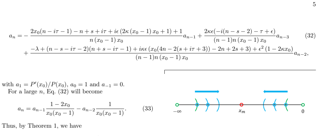
Calculate the connection coefficients of P in 0 = C in ∞P in ∞ + C out ∞ P out ∞ , (35) P out ∞ = C in 0 P in 0 + C out 0 P out 0 (36) from the values and derivatives of each function at the match point xm. Then, for x < xm and x > xm, we can use Eq. (35) and Eq. (36) to give the results of P in 0 and P out ∞ , respectively
-
[6]
Obtain Rin and Rup at arbitrary x <0 by Rin = T Pin 0 , (37) Rup = T Pout ∞ . (38) FIG. 1. A schematic diagram that describes the process of the global solution construction. The match point xm can be selected as an arbitrary number smaller than 0. See also Fig. 1, which provides a schematic overview of the procedure above. In principle, the match point x...
-
[7]
Thus, for the solutions v1 and v2 of Eq
+ t2 1, (E5) and s(x) is a smooth function whose explicit form is use- less for the following proof. Thus, for the solutions v1 and v2 of Eq. (E4), the new Wronskian constant Wn reads Wn(v1, v2) =I(v1, v2, x) exp Z f (x) − h′(x) h(x) dx =h(x)I(w1, w2, x) exp Z f (x)dx − ln h(x) =I(w1, w2, x) exp Z f (x)dx =W(w1, w2) (E6) We then discuss the transformation...
-
[8]
R. Abbott et al. (LIGO Scientific, VIRGO, and KAGRA Collaborations), Gwtc-3: Compact binary coalescences observed by ligo and virgo during the second part of the third observing run (2021), arXiv:2111.03606 [gr-qc]
arXiv 2021
Show all 49 references
-
[9]
B. P. Abbott, R. Abbott, et al. (LIGO Scientific Collab- oration and Virgo Collaboration), Observation of grav- itational waves from a binary black hole merger, Phys. Rev. Lett. 116, 061102 (2016)
2016
-
[10]
Hu and Y.-L
W.-R. Hu and Y.-L. Wu, The Taiji Program in Space for gravitational wave physics and the nature of gravity, National Science Review 4, 685 (2017), https://academic.oup.com/nsr/article- pdf/4/5/685/31566708/nwx116.pdf
2017
-
[11]
Amaro-Seoane et al
P. Amaro-Seoane et al. (LISA Collaboration), Laser interferometer space antenna (2017), arXiv:1702.00786 [astro-ph.IM]
2017 arXiv
-
[12]
Luo, L.-S
J. Luo, L.-S. Chen, H.-Z. Duan, Y.-G. Gong, S. Hu, J. Ji, Q. Liu, J. Mei, V. Milyukov, M. Sazhin, C.-G. Shao, V. T. Toth, H.-B. Tu, Y. Wang, Y. Wang, H.-C. Yeh, M.-S. Zhan, Y. Zhang, V. Zharov, and Z.-B. Zhou, Tianqin: a space-borne gravitational wave detector, Classical and Q...
2016
-
[13]
Amaro-Seoane et al., Astrophysics with the laser interfer- ometer space antenna, Living Reviews in Relativity 26, 2 (2023)
2023
-
[14]
Babak, J
S. Babak, J. Gair, A. Sesana, E. Barausse, C. F. Sop- uerta, C. P. L. Berry, E. Berti, P. Amaro-Seoane, A. Pe- titeau, and A. Klein, Science with the space-based in- terferometer lisa. v. extreme mass-ratio inspirals, Phys. Rev. D 95, 103012 (2017)
2017
-
[15]
Amaro Seoane et al
P. Amaro Seoane et al. , The effect of mission duration on lisa science objectives, General Relativity and Gravi- tation 54, 3 (2021)
2021
-
[16]
Laghi, N
D. Laghi, N. Tamanini, W. Del Pozzo, A. Sesana, J. Gair, S. Babak, and D. Izquierdo-Villalba, Gravitational- wave cosmology with extreme mass-ratio inspirals, Monthly Notices of the Royal Astronomical Society 508, 4512 (2021), https://academic.oup.com/mnras/article- pdf/508/3/...
2021
-
[17]
Cardoso, K
V. Cardoso, K. Destounis, F. Duque, R. P. Macedo, and A. Maselli, Gravitational waves from extreme-mass-ratio systems in astrophysical environments, Phys. Rev. Lett. 129, 241103 (2022)
2022
-
[18]
Askar, C
A. Askar, C. Belczynski, et al., Black holes, gravitational waves and fundamental physics: a roadmap, Classical and Quantum Gravity 36, 143001 (2019)
2019
-
[19]
Barausse et al
E. Barausse et al. , Prospects for fundamental physics with lisa, General Relativity and Gravitation 52, 81 (2020)
2020
-
[20]
M. L. Katz, A. J. K. Chua, L. Speri, N. Warburton, and S. A. Hughes, Fast extreme-mass-ratio-inspiral wave- forms: New tools for millihertz gravitational-wave data analysis, Phys. Rev. D 104, 064047 (2021)
2021
-
[21]
Pound and B
A. Pound and B. Wardell, Black hole perturbation the- ory and gravitational self-force, in Handbook of Gravi- tational Wave Astronomy , edited by C. Bambi, S. Kat- sanevas, and K. D. Kokkotas (Springer Singapore, Sin- gapore, 2020) pp. 1–119
2020
-
[22]
S. A. Teukolsky, Perturbations of a Rotating Black Hole. I. Fundamental Equations for Gravitational, Electromag- netic, and Neutrino-Field Perturbations, apj 185, 635 (1973)
1973
-
[23]
W. H. Press and S. A. Teukolsky, Perturbations of a Ro- tating Black Hole. II. Dynamical Stability of the Kerr Metric, apj 185, 649 (1973)
1973
-
[24]
S. A. Teukolsky and W. H. Press, Perturbations of a ro- tating black hole. III. Interaction of the hole with gravita- tional and electromagnetic radiation., Astrophys. J. 193, 443 (1974)
1974
-
[25]
Drasco and S
S. Drasco and S. A. Hughes, Gravitational wave snap- shots of generic extreme mass ratio inspirals, Phys. Rev. D 73, 024027 (2006)
2006
-
[26]
E. W. Leaver, Solutions to a generalized spheroidal wave equation: Teukolsky’s equations in general rel- 15 ativity, and the two-center problem in molecular quantum mechanics, Journal of Mathematical Physics 27, 1238 (1986), https://pubs.aip.org/aip/jmp/article- pdf/27/5/1238/...
1986
-
[27]
S. Mano, H. Suzuki, and E. Takasugi, Analytic so- lutions of the teukolsky equation and their low fre- quency expansions, Progress of Theoretical Physics 95, 1079 (1996), https://academic.oup.com/ptp/article- pdf/95/6/1079/5282662/95-6-1079.pdf
1996
-
[28]
Fujita and H
R. Fujita and H. Tagoshi, New numerical methods to evaluate homogeneous solutions of the teukol- sky equation, Progress of Theoretical Physics 112, 415 (2004), https://academic.oup.com/ptp/article- pdf/112/3/415/5382220/112-3-415.pdf
2004
-
[29]
Fujita and H
R. Fujita and H. Tagoshi, New numerical methods to evaluate homogeneous solutions of the teukolsky equation. ii: — solutions of the continued fraction equation —, Progress of Theoretical Physics 113, 1165 (2005), https://academic.oup.com/ptp/article- pdf/113/6/1165/5285582/113...
2005
-
[30]
Sasaki and T
M. Sasaki and T. Nakamura, The regge-wheeler equation with sources for both even and odd parity perturbations of the schwarzschild geometry, Physics Letters A 87, 85 (1981)
1981
-
[31]
Sasaki and T
M. Sasaki and T. Nakamura, A class of new perturbation equations for the kerr geometry, Physics Letters A89, 68 (1982)
1982
-
[32]
Sasaki and T
M. Sasaki and T. Nakamura, Gravitational radiation from a kerr black hole. i. formulation and a method for numerical analysis, Progress of Theoretical Physics 67, 1788 (1982), https://academic.oup.com/ptp/article- pdf/67/6/1788/5332324/67-6-1788.pdf
1982
-
[33]
S. A. Hughes, Computing radiation from kerr black holes: Generalization of the sasaki-nakamura equation, Phys. Rev. D 62, 044029 (2000)
2000
-
[34]
R. K. L. Lo, Recipes for computing radiation from a kerr black hole using a generalized sasaki-nakamura formal- ism: Homogeneous solutions, Phys. Rev. D 110, 124070 (2024)
2024
-
[35]
Chen and J
C. Chen and J. Jing, Gravitational wave fluxes on generic orbits in near-extreme kerr spacetime: Higher spin and large eccentricity, Science China Physics, Mechanics & Astronomy 67, 110411 (2024)
2024
-
[36]
Elaydi, Asymptotic behavior of difference equations, in An Introduction to Difference Equations (Springer New York, New York, NY, 2005) pp
S. Elaydi, Asymptotic behavior of difference equations, in An Introduction to Difference Equations (Springer New York, New York, NY, 2005) pp. 335–395
2005
-
[37]
DLMF, NIST Digital Library of Mathematical Functions, https://dlmf.nist.gov/2.7.i, Release 1.2.4 of 2025- 03-15, f. W. J. Olver, A. B. Olde Daalhuis, D. W. Lozier, B. I. Schneider, R. F. Boisvert, C. W. Clark, B. R. Miller, B. V. Saunders, H. S. Cohl, and M. A. McClain, eds
2025
-
[38]
D. L. Bosley, A technique for the numerical verification of asymptotic expansions, SIAM Review 38, 128 (1996), https://doi.org/10.1137/1038006
1996 doi
-
[39]
A. B. O. Daalhuis and F. W. J. Olver, Exponentially improved asymptotic solutions of ordinary differential equations. ii. irregular singularities of rank one, Pro- ceedings of the Royal Society of London. Series A: Mathematical and Physical Sciences 445, 39 (1994), https://roy...
1994
-
[40]
E. J. Weniger, Nonlinear sequence transformations for the acceleration of convergence and the summation of di- vergent series, Computer Physics Reports10, 189 (1989)
1989
-
[41]
Berti, V
E. Berti, V. Cardoso, and M. Casals, Eigenvalues and eigenfunctions of spin-weighted spheroidal harmonics in four and higher dimensions, Phys. Rev. D 73, 024013 (2006)
2006
-
[42]
Olver, 10 - differential equations with a parameter: Expansions in elementary functions, in Asymptotics and Special Functions, edited by F
F. Olver, 10 - differential equations with a parameter: Expansions in elementary functions, in Asymptotics and Special Functions, edited by F. Olver (Academic Press,
-
[43]
Ferreira, J
C. Ferreira, J. L. Lopez, and E. P. Sinusia, Olver’s asymp- totic method: a special case (2014), arXiv:1406.1613 [math.CA]
2014 arXiv
-
[44]
Black Hole Perturbation Toolkit, (bhptoolkit.org)
-
[45]
R. K. L. Lo, L. Sabani, and V. Cardoso, Quasinormal modes and excitation factors of Kerr black holes, Phys. Rev. D 111, 124002 (2025), arXiv:2504.00084 [gr-qc]
2025 arXiv
-
[46]
E. W. Leaver and S. Chandrasekhar, An analytic representation for the quasi-normal modes of kerr black holes, Proceedings of the Royal Society of London. A. Mathematical and Physical Sciences 402, 285 (1985), https://royalsocietypublishing.org/doi/pdf/10.1098/rspa.1985.0119
1985
-
[47]
S. A. Hughes, Evolution of circular, nonequatorial orbits of kerr black holes due to gravitational-wave emission, Phys. Rev. D 61, 084004 (2000)
2000
-
[48]
G. B. Cook and M. Zalutskiy, Gravitational perturba- tions of the kerr geometry: High-accuracy study, Phys. Rev. D 90, 124021 (2014)
2014
-
[49]
OL WR, Numerical solution of second-order linear dif- ference equations, J
F. OL WR, Numerical solution of second-order linear dif- ference equations, J. Res. Nat. Bur. Standards B 71
Reviewed August 6, 2026 · model on record in the stance chip above.
Discussion (0). Continue with ORCID to comment.