A sub-modular receding horizon solution for mobile multi-agent persistent monitoring

Navid Rezazadeh; Solmaz S. Kia

REVIEW 4 major objections 6 minor 40 references

A sub-modular receding horizon solution for mobile multi-agent persistent monitoring

T0 review · 4 major / 6 minor · reviewed 2026-08-14 · deepseek-v4-flash

Challenge this review Re-run · record.json Download PDF Read on arXiv ↗ Review JSON

Pith's one-line read The paper proves that the persistent-monitoring dispatch utility is monotone submodular, so a sequential greedy policy over agents achieves at least half the optimal reward in polynomial time.

desk verdict The concave-reward patrolling greedy is a good idea and likely correct, but the submodularity proof as written doesn't cover interleaved agent visits and Corollary 4.1 has a sign error; worth refereeing, not accepting as-is. read the letter →

arxiv 1908.04425 v3 pith:TRLHXIO7 submitted 2019-08-12 cs.MA cs.RO

Navid Rezazadeh , Solmaz S. Kia This is my paper · ORCID

classification cs.MAcs.RO MSC 90C2768W25

keywords persistentmonitoringmulti-agentpatrollingsubmodularoptimizationsequentialgreedyalgorithmrecedinghorizonnodalimportancemobilesensorsoptimalitygap

verification ladder T0 review T1 audit T2 compute T3 formal

The pith

A machine-rendered reading of the paper's core claim, the machinery that carries it, and where it could break.

The reading

This paper studies persistent monitoring, where a team of mobile agents visits interconnected nodes and each node's reward grows concavely since its last visit and resets to zero on a visit. The question is which nodes to visit, when, and by which agent to maximize total reward over the mission horizon, and the paper shows that the exact answer is NP-hard and exponential in the number of agents and horizon length. The central claim is that the total-reward utility, viewed as a function of the chosen set of agent policies, is monotone increasing and submodular, meaning the marginal value of any additional policy never increases as more policies are already in the set. Because of this, the sequential greedy algorithm that assigns one policy per agent runs in polynomial time and is guaranteed to collect at least half of the optimal reward. A receding-horizon implementation plus a nodal-importance term for reward beyond the current horizon preserves that same guarantee and gives agents a reason to head toward distant high-reward regions.

What carries the argument

The load-bearing object is the augmented utility $\bar{R}(\bar{P})$ in (5), defined over policy sets subject to a partition-matroid constraint (at most one policy per agent). It turns an NP-hard dynamic scheduling problem into a monotone submodular set-function maximization, which is exactly the setting where the sequential greedy algorithm carries a $1/2$ optimality gap. The technical engine proving submodularity is the representation of a node's contribution as $\sum_j \psi_v(\Delta t^v_j)$, where $\Delta t^v_j$ are the gaps between consecutive visits to node $v$, together with concatenation lemmas (A.2 and A.3) based on Karamata's inequality that compare marginal gains of adding a policy to a smaller versus a larger set. The nodal-importance term $\mathcal{L}(v,w,\hat{t},i)$ measures the reward concentration within radius $r$ of an anchor node, normalized by travel time, and is designed to be modular so that adding it does not disturb submodularity; the paper notes its resemblance to a terminal cost in model predictive control.

What would settle it

Simulate a single node with a concave reward and three visit schedules chosen so that policy q inserts a visit between two visits of the existing set; compute the marginal gain $\Delta R(q|Q_1)$ for a smaller set $Q_1$ and a larger set $Q_2$. If any such schedule yields a marginal gain for $Q_1$ smaller than for $Q_2$, submodularity fails and the $1/2$ bound collapses. A positive check across all small exhaustive cases, for example with three or four visits, would support the missing lemma.

Watch

Extended reading notes

Core claim

The paper's discovery, stated on its own terms, is that the persistent-monitoring dispatch problem, despite being NP-hard, can be approximately solved with a constant factor because its utility is well behaved. For a selected policy set $\bar{P}$, the utility is $R(\bar{P}) = \sum_{p\in\bar{P}}\sum_{l=1}^{n_p} R_{V_p(l)}(T_p(l))$, the sum of all node rewards collected at visit times, with each node reward of the form $\psi_v(t-\bar{t}_v)$ for an increasing concave $\psi_v$. Theorem 3.1 asserts that this utility, augmented as $\bar{R}(\bar{P}) = R(\bar{P}) + \alpha\sum_{p\in\bar{P}}\max_{v\in\bar{V}}\mathcal{L}(v,p)$ with relative nodal importance $\mathcal{L}$ and any $\alpha\ge0$, is a monotone increasing and submodular set function over the feasible policy set under the constraint that at most one policy is chosen per agent. Theorem 3.2 then concludes that Algorithm 1, a sequential greedy pass over agents, returns a policy set $\bar{P}$ with $\bar{R}(\bar{P}) \ge \tfrac12 \bar{R}(P^\star)$, where $P^\star$ is the optimal solution of (4). The proof route rewrites each node's reward as a sum over gaps between consecutive visits and invokes Karamata-based lemmas to show diminishing returns.

Load-bearing premise

The whole guarantee rests on the reward staying submodular when a new agent's visits are inserted between existing visits, but the proof only covers insertions appended after the current visit sequence, so the arbitrarily interleaved case is assumed rather than proved.

Editorial extensions

If this is right

A user can replace exponential search over all policy combinations with one greedy pass over agents and still receive a guaranteed half-optimality certificate for the augmented utility.
The $1/2$ guarantee survives the receding-horizon shortening of plans and the addition of the nodal-importance term with any nonnegative weight $\alpha$.
In decentralized execution with full information sharing, such as a Hamiltonian communication route or non-overlapping cloud time slots, the same $1/2$ gap holds.
When message dropouts make the information graph incomplete, the optimality gap degrades to $1/(M-\omega(G_I)+2)$, where $\omega(G_I)$ is the clique number of the information graph.
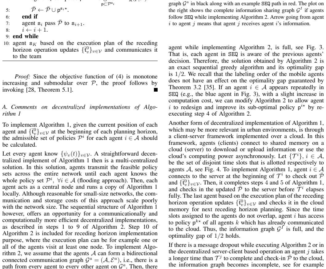
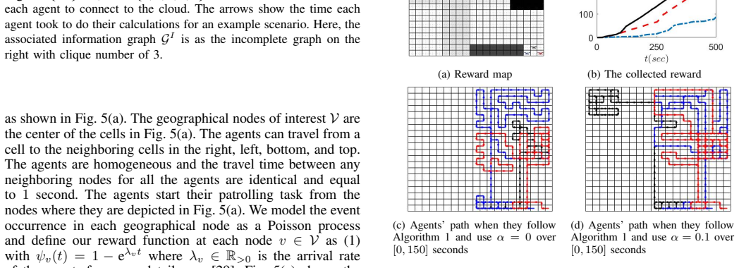
For event-detection rewards of the form $1-e^{\lambda_v t}$ (Poisson arrivals), the nodal-importance term steers agents toward high-rate clusters beyond the current planning horizon, as the simulation demonstrates.

Reading between the lines

Editorial extensions of the paper, not claims the author makes directly.

The same submodularity machinery should extend to heterogeneous travel times and agent-specific scanning delays, since the per-node visit-time sequence argument does not appear to use homogeneity; testing this is a direct next step the paper does not pursue.
If submodularity holds across arbitrarily interleaved visits, the approach should generalize to stochastic rewards or time-varying $\psi_v$ as long as concavity and reset-on-visit are preserved, but the paper makes no such claim.
The receding-horizon-plus-terminal-importance structure suggests a bridge to model predictive control theory: tightening the terminal cost could yield stability-style guarantees on long-run visit frequencies, not just horizon-by-horizon reward.
The choice of anchor nodes $\bar{V}$ is left as a design parameter, so an adaptive anchor-selection rule based on current reward gradients is a natural testable extension that the paper does not analyze.

Share X Bluesky LinkedIn Reddit HN

Signed reviews

No signed human review yet.

Editorial analysis

A structured set of objections, weighed in public.

Desk editor's note, referee report, and a circularity audit.

Desk Editor's Note

read the letter

Short version: the paper's central claim—submodularity of the concave-interval reward, hence a polynomial-time greedy with 1/2 gap—is almost certainly true, but the written proof doesn't cover the actual multi-agent case and there is a sign error in a corollary. I would not accept it as-is; I would send it to referees and ask for a revised proof.

The new idea is worth stating clearly. Previous patrolling work mostly used idle time, which is a linear reward. Here the reward per node is a concave increasing function of time since last visit, which is the right model for event detection. The utility is a set function over agent policies, the authors prove monotonicity/submodularity, and then the partition-matroid constraint gives the Fisher–Nemhauser–Wolsey 1/2 gap. The receding-horizon 'nodal importance' term, which adds a terminal-cost-like reward for being near high-value regions, is a sensible heuristic, and the decentralized greedy is a nice addition. The simulation illustrates the benefit of the terminal term over a plain look-ahead greedy.

The soft spots are real and they sit in the load-bearing proof. Theorem 3.1 relies on Lemmas A.2 and A.3, but those lemmas are proved for the case where the new visits are concatenated after the existing visits at a node. In the actual problem, adding an agent policy inserts visits at times that interleave with visits from other agents. The proof never handles that. Independent reasoning says the statement is true: splitting an interval into two parts with lengths x and y produces incremental reward ψ(x)+ψ(y)−ψ(x+y), which is increasing in x and y for concave increasing ψ, so the marginals do diminish. The paper does not supply that argument. On top of that, Corollary 4.1 is stated in the wrong direction: the printed inequality is false already for f(t)=√t, a=b=1, c=d=4. The proof actually concludes the opposite, which is the direction Lemma A.3 needs, so it is probably a typo, but a typo in a lemma that Theorem 3.1 leans on is not nothing.

The simulation is a single scenario without error bars, so it is suggestive rather than evidence. The NP-hardness claim is standard.

All in all, the engineering and the high-level result are solid, the proof as written is not. This paper deserves a serious referee, but the referee should be explicitly asked to check the corrected submodularity proof under interleaving and the direction of Corollary 4.1. I would not cite the current version.

Referee Report

4 major / 6 minor

Summary. The paper addresses persistent monitoring of a finite set of graph nodes by heterogeneous mobile agents. Each node carries a concave, increasing reward that resets upon a visit, and the dispatch problem is to select one policy per agent to maximize the total collected reward over a mission horizon. The authors state that the problem is NP-hard, prove in Theorem 3.1 that the utility, augmented with a nodal-importance term, is monotone submodular, and use this to claim a 1/2 optimality gap for their sequential greedy algorithm (Theorem 3.2), implemented in a receding horizon and decentralized fashion. A simulation study illustrates the method.

Significance. If the submodularity claim is correct, the paper offers a polynomial-time dispatch algorithm with a constant-factor approximation guarantee for a persistent monitoring problem with concave resetting rewards, a genuinely useful extension of submodular maximization to dynamic scheduling. The use of Karamata's inequality to study visit-interval rewards is an interesting technique and the nodal-importance term is a sensible remedy for receding-horizon shortsightedness. However, the written proof has load-bearing gaps: the auxiliary lemmas cover only concatenated visit sequences, not the interleaved insertions that arise in the actual multi-agent problem, and Corollary 4.1 is stated and proved with the wrong inequality direction. The central claim is plausible and likely repairable, but the current manuscript does not provide a gap-free derivation of the advertised 1/2 guarantee.

major comments (4)

[Theorem 3.1 proof and Appendix Lemmas A.2, A.3] The submodularity proof is load-bearing: Theorem 3.2's 1/2 gap rests entirely on it. Yet Lemmas A.2 and A.3 are proved only for concatenated visit sequences of the form (t)⊕(u) or (v)⊕(u), where the newly added visits are appended after the existing visits. In the actual problem, adding a policy q to a set Q inserts visits at arbitrary times between previously scheduled visits at each node. The proof of Theorem 3.1 does not address interleaved insertion, so the marginal-diminishing inequality ΔR̄(q|Q1) ≥ ΔR̄(q|Q2) is not established for the feasible policy sets of (4). This gap must be closed, for example by proving that the per-node insertion benefit F(u,v)=ψ(u)+ψ(v)−ψ(u+v) is nondecreasing in both arguments for concave increasing ψ, or by a direct generalization of Lemmas A.2 and A.3 to interleaved sequences.
[Corollary 4.1 and Lemma A.3] Corollary 4.1 is stated with the wrong inequality direction. As printed, it claims f(c)+f(d)−f(c+d) ≤ f(a)+f(b)−f(a+b) for 0≤a≤c and 0≤b≤d, but the reverse inequality is true for increasing concave f, and a counterexample is f(t)=√t, a=b=1, c=d=4 (the left side is about 1.172, the right side about 0.586). The proof concludes the same backward inequality, so both the statement and the derivation must be corrected. Lemma A.3 uses Corollary 4.1 to conclude ΔSp ≥ 0, and that conclusion requires the opposite, correct direction. This is therefore not a harmless typo in one line; it affects the validity of Lemma A.3 and hence of Theorem 3.1 as written.
[Assumption 1 and Eq. (2)] There is an inconsistency between the model and the objective function. Assumption 1 states that if more than one agent arrives at node v at the same time, the team still collects only R_v(t). However, the utility in Eq. (2) is a sum over every visit of every policy, so simultaneous visits would double-count the reward. As written, the optimization problem (3) maximizes an objective that does not match the described monitoring reward. The authors should either reformulate the utility to count each distinct reward-earning event once, or explicitly restrict the feasible set to policies with no simultaneous visits and explain how the submodularity proof extends to that restriction.
[Theorem 3.1 proof, monotonicity step] The monotonicity portion of the proof of Theorem 3.1 contains mismatched indices. The displayed expression compares a sum over (t_v(Q2∪q)) with a sum over (t_v(Q2)), yet the conclusion is stated as ΔR(p|Q1) ≥ 0. Neither the indexing nor the use of Lemma A.2 (which applies to concatenated sequences) establishes the intended monotonicity of R with respect to adding q to Q1. This part of the proof needs to be rewritten together with the interleaving fix described above.

minor comments (6)

[Lemma A.2 proof] In the final displayed inequality of Lemma A.2, the index "n+1−1" is unclear and appears to be a typo; it should likely read "n+l−1" or the intended upper limit should be stated clearly.
[Lemma A.3 proof] In the telescoping-sum equation at the end of Lemma A.3, the second term in parentheses should be (g((t)^n_1)−g((v)^m_1)) or equivalent; as printed it repeats g((v)^m_1) and does not telescope correctly.
[Eq. (2)] Equation (2) contains a duplicated fragment: "R : 2P→ R>0 is ¯P ⊂P, the utility function R : 2P→ R>0 is" appears twice in a row, which disrupts the definition.
[Section III-A] The definition of the clique number is incorrect: "the number of the nodes in the largest sub-graph such that adding an edge will cause a cycle" is not the clique number. The clique number is the size of the largest complete subgraph; the statement should be corrected.
[Algorithm 2 discussion] The sentence describing what happens when an agent appears repeatedly in SEQ says the agent can "redesign and improve its sub-optimal policy" but does not specify the mechanism or its effect on the optimality gap. This should be made precise or removed.
[Numerical example] Given the inconsistency between Assumption 1 and Eq. (2), the simulation section should state explicitly how simultaneous arrivals are resolved in the implementation.

Circularity Check

0 steps flagged · score 0.0 of 10

No significant circularity: the 1/2 optimality gap is derived from a submodularity proof based on Karamata-type lemmas and the external Fisher–Nemhauser–Wolsey bound, not from fitted inputs or self-citation.

full rationale

The derivation chain is self-contained. Theorem 3.1 asserts submodularity of the augmented reward Rbar in (5); its proof derives the marginal-diminishing property for the visit-reward part from Lemmas A.2 and A.3, which are proven from Karamata's inequality, and observes that the nodal-importance term is modular and hence preserves submodularity. Theorem 3.2 then invokes the classical Fisher, Nemhauser and Wolsey result [28] to obtain the 1/2 approximation gap for the sequential greedy algorithm. No parameter is fitted to data and then renamed as a prediction, and no claim reduces by definition to its own input. The self-citation [29] is used only as a preliminary workshop reference and for details of the reward model in the simulation, not as a load-bearing justification of the central theorems. The known proof gaps noted by the reader—Lemmas A.2 and A.3 are proved only for concatenated visit sequences while interleaved visits can occur in the multi-agent problem, and Corollary 4.1 is stated with an apparently reversed inequality—are correctness concerns about the written proof, not circularity. Therefore the circularity score is 0.

Assumptions & free parameters 2 free parameters · 4 assumptions · 0 invented entities

The central claim rests on the concavity-and-reset reward model, the Karamata-based submodularity lemmas, and the fixed-horizon interpretation of the nodal-importance term. No free parameters are fitted to data to obtain the main guarantee; α and r are user-chosen heuristic parameters. No new physical entities are introduced. The main unstated mathematical assumption is that the concatenation lemmas extend to interleaved insertion of new policy visits.

free parameters (2)

α (nodal importance weight) = 0.1 in simulation
Hand-chosen weight balancing collected reward and terminal importance; the theorem holds for any α≥0, so it is not fitted to make the proof work.
r (nodal importance radius) = not specified numerically
Radius of the neighborhood used to define L(v,τ,r); must be chosen by the user, and the paper gives no guidance in the main text.

assumptions (4)

domain assumption Each node's reward ψ_v(t) is nonnegative, concave, increasing, with ψ_v(0)=0, and resets to zero after an agent's visit (Eq. 1).
This is the reward model underlying the utility (2) and the submodularity claim. It is stated in Section II and used throughout the proof of Theorem 3.1.
standard math Karamata's inequality (majorization) applies to the rearranged inter-visit intervals (Lemma A.1).
Used to prove Lemmas A.2 and A.3 in the appendix, which support Theorem 3.1.
ad hoc to paper The relative nodal importance L(v,p) is evaluated using the last-visit times {t_v^0} fixed at the start of the planning horizon and does not change as policies are added in the greedy selection (Eq. 5).
This makes the second summand in (5) modular; if t_v were updated during selection, the function would not decompose as assumed and the proof would need amendment.
domain assumption Assumption 1: an agent scans immediately on arrival; if multiple agents arrive simultaneously, the team collects only one reward; Assumption 2: agents only move along edges of the graph.
These define the feasible policy set and avoid double counting rewards; they are standard for patrolling models.

how reviews work

0 comments

Cite this review

Pith. "Pith review of A sub-modular receding horizon solution for mobile multi-agent persistent monitoring." pith.science (2026). https://pith.science/paper/TRLHXIO7

@misc{pith2026190804425,
  author       = {Pith},
  title        = {Pith review of: A sub-modular receding horizon solution for mobile multi-agent persistent monitoring},
  year         = {2026},
  howpublished = {\url{https://pith.science/paper/TRLHXIO7}},
  note         = {Machine review of arXiv:1908.04425}
}

read the original abstract

We study the problem of persistent monitoring of a finite number of inter-connected geographical nodes by a group of heterogeneous mobile agents. We assign to each geographical node a concave and increasing reward function that resets to zero after an agent's visit. Then, we design the optimal dispatch policy of which nodes to visit at what time and by what agent by finding a policy set that maximizes a utility that is defined as the total reward collected at visit times. We show that this optimization problem is NP-hard and its computational complexity increases exponentially with the number of the agents and the length of the mission horizon. By showing that the utility function is a monotone increasing and submodular set function of agents' policy, we proceed to propose a suboptimal dispatch policy design with a known optimality gap. To reduce the time complexity of constructing the feasible search set and also to induce robustness to changes in the operational factors, we perform our suboptimal policy design in a receding horizon fashion. Then, to compensate for the shortsightedness of the receding horizon approach for reward distribution beyond the feasible policies of the agents over the receding horizon, we add a new term to our utility, which provides a measure of nodal importance beyond the receding horizon's sight. This term gives the policy design an intuition to steer the agents towards the nodes with higher rewards on the patrolling graph. Finally, we discuss how our proposed algorithm can be implemented in a decentralized manner. A simulation study demonstrates our results.

Figures

Figures reproduced from arXiv: 1908.04425 by the authors.

**Figure 1.** Examples of a set of geographical nodes of interest and the edges between them. Finite number of nodes to monitor in a city can be restricted to some particular scanning zones (the picture on the left) or the cell partitioned map of the city (the picture on the right). The mobile agents are confined to a set of pre-specified edges E ⊂ V × V, e.g., aerial or ground corridors, to traverse from one node to another, see… view at source ↗

**Figure 2.** An agent has two possible routes to take over the designated receding horizon. The nodes’ color intensity shows their reward value. The blue route offers a higher reward over the receding horizon but it puts the agent close to an area with a lower amount of reward, while the red route results in lower total reward over the receding horizon but puts the agent near an area with higher amount of reward. however, the mo… view at source ↗

**Figure 3.** The plot on the left shows the bi-directional communication graph G a in black along with an example SEQ path in red. The plot on the right shows the complete information sharing graph G I if agents follow SEQ while implementing Algorithm 2. Arrow going from agent i to agent j means that agent j receives agent i’s information. agent while implementing Algorithm 2, is full, see [PITH_FULL_IMAGE:figures/full_fig_p005… view at source ↗

Figures from the paper (3 more)

**Figure 4.** Figure 4: Then, the corresponding decentralized implementation [PITH_FULL_IMAGE:figures/full_fig_p005_4.png]

**Figure 4.** Figure 4: {T i }i∈A, A = {1, 2, 3, 4, 5} are the time slots allotted to each agent to connect to the cloud. The arrows show the time each agent took to do their calculations for an example scenario. Here, the associated information graph G I is as the incomplete graph on the rig…

**Figure 5.** Figure 5: (c) shows. However, there are other important regions with higher values that are farther away, especially the area on the left top corner which is separated by a low rate stripe from where agents start. Incorporating nodal importance, as (a) Reward map (b) The collect…

Discussion (0). Continue with ORCID to comment.

Reference graph

Works this paper leans on

40 extracted references · 39 canonical work pages

[1]

Coverage control for mobile sensing networks,

J. Cortes, S. Martinez, T. Karatas, and F. Bullo, “Coverage control for mobile sensing networks,” IEEE Tran. on Automatic Control , vol. 20, no. 2, pp. 243–255, 2004

work page 2004
[2]

Near-optimal observation selection using submodular functions,

A. Krause and C. Guestrin, “Near-optimal observation selection using submodular functions,” in American Association for Artiﬁcial Intelli- gence, vol. 7, pp. 1650–1654, 2007

work page 2007
[3]

Near-optimal sensor placements in Gaussian processes: Theory, efﬁcient algorithms and empirical stud- ies,

A. Krause, A. Singh, and C. Guestrin, “Near-optimal sensor placements in Gaussian processes: Theory, efﬁcient algorithms and empirical stud- ies,” Journal of Machine Learning Research , vol. 9, no. Feb, pp. 235– 284, 2008

work page 2008
[4]

Decentralized, adaptive coverage control for networked robots,

M. Schwager, D. Rus, and J. Slotine, “Decentralized, adaptive coverage control for networked robots,” The Int. Journal of Robotics Research , vol. 28, no. 3, pp. 357–375, 2009

work page 2009
[5]

Gossip coverage control for robotic networks: Dynamical systems on the space of partitions,

F. Bullo, R. Carli, and P. Frasca, “Gossip coverage control for robotic networks: Dynamical systems on the space of partitions,” SIAM Journal on Control and Optimization , vol. 50, no. 1, pp. 419–447, 2012

2012
[6]

Multi-agents adaptive estimation and coverage control using gaussian regression,

A. Carron, M. Todescato, R. Carli, L. Schenato, and G. Pillonetto, “Multi-agents adaptive estimation and coverage control using gaussian regression,” in 2015 European Control Conference (ECC) , pp. 2490– 2495, IEEE, 2015

work page 2015
[7]

Multi-robots gaussian estimation and coverage control: From client– server to peer-to-peer architectures,

M. Todescato, A. Carron, R. Carli, G. Pillonetto, and L. Schenato, “Multi-robots gaussian estimation and coverage control: From client– server to peer-to-peer architectures,” Automatica, vol. 80, pp. 284–294, 2017

work page 2017
[8]

A distributed service-matching coverage via heterogeneous mobile agents

Y . Chung and S. S. Kia, “A distributed service-matching cov- erage via heterogeneous mobile agents,” 2020. available at https://arxiv.org/pdf/2009.11943.pdf

work page Pith review arXiv 2020

Show all 40 references

[9]

A survey on technologies for automatic forest ﬁre monitoring, detection, and ﬁghting using unmanned aerial vehicles and remote sensing techniques,

C. Yuan, Y . Zhang, and Z. Liu, “A survey on technologies for automatic forest ﬁre monitoring, detection, and ﬁghting using unmanned aerial vehicles and remote sensing techniques,” Canadian Journal of Forest Research, vol. 45, no. 7, pp. 783–792, 2015

2015
[10]

Wireless sensor networks based pipeline vandalisation and oil spillage monitoring and detection: main beneﬁts for nigeria oil and gas sectors,

N. Henry and O. Henry, “Wireless sensor networks based pipeline vandalisation and oil spillage monitoring and detection: main beneﬁts for nigeria oil and gas sectors,” The SIJ Tran. on Computer Science Engineering & its Applications (CSEA) , vol. 3, no. 1, pp. 1–6, 2015

2015
[11]

An improved approach for predicting the distribution of rare and endangered species from occurrence and pseudo-absence data,

R. Engler, A. Guisan, and L. Rechsteiner, “An improved approach for predicting the distribution of rare and endangered species from occurrence and pseudo-absence data,” J. of Applied Ecology , vol. 41, no. 2, pp. 263–274, 2004

2004
[12]

Detection of incidents and events in urban networks,

T. Thomas and E. van Berkum, “Detection of incidents and events in urban networks,” IET Intelligent Transport Systems , vol. 3, no. 2, pp. 198–205, 2009

2009
[13]

Reducibility among combinatorial problems,

R. Karp, “Reducibility among combinatorial problems,” in Complexity of computer computations , pp. 85–103, Springer, 1972

1972
[14]

Multi-agent pa- trolling: An empirical analysis of alternative architectures,

A. Machado, G. Ramalho, J. Zucker, and A. Drogoul, “Multi-agent pa- trolling: An empirical analysis of alternative architectures,” in Interna- tional Workshop on Multi-Agent Systems and Agent-Based Simulation , pp. 155–170, 2002

2002
[15]

Recent advances on multi-agent patrolling,

A. Almeida, G. Ramalho, H. Santana, P. Tedesco, T. Menezes, V . Corru- ble, and Y . Chevaleyre, “Recent advances on multi-agent patrolling,” in Brazilian Symposium on Artiﬁcial Intelligence , pp. 474–483, Springer, 2004

2004
[16]

Theoretical analysis of the multi-agent patrolling prob- lem,

Y . Chevaleyre, “Theoretical analysis of the multi-agent patrolling prob- lem,” in Intelligent Agent Technology, pp. 302–308, IEEE, 2004

2004
[17]

On cooperative patrolling: Op- timal trajectories, complexity analysis, and approximation algorithms,

F. Pasqualetti, A. Franchi, and F. Bullo, “On cooperative patrolling: Op- timal trajectories, complexity analysis, and approximation algorithms,” IEEE Tran. on Robotics , vol. 28, no. 3, pp. 592–606, 2012

2012
[18]

Persistent monitoring of events with stochastic arrivals at multiple stations,

J. Yu, S. Karaman, and D. Rus, “Persistent monitoring of events with stochastic arrivals at multiple stations,”IEEE Tran. on Robotics, vol. 31, no. 3, pp. 521–535, 2015

2015
[19]

Persistent surveillance of transient events with unknown statistics,

M. Donahue, G. Rosman, K. Kotowick, D. Rus, and C. Baykal, “Persistent surveillance of transient events with unknown statistics,” tech. rep., MIT Lincoln Laboratory Lexington United States, 2016

2016
[20]

Multi-robot routing for persistent monitoring with latency constraints,

A. Asghar, S. Smith, and S. Sundaram, “Multi-robot routing for persistent monitoring with latency constraints,” arXiv preprint arXiv:1903.06105, 2019

1903 arXiv
[21]

Distributed on-line dynamic task assignment for multi-robot patrolling,

A. Farinelli, L. Iocchi, and D. Nardi, “Distributed on-line dynamic task assignment for multi-robot patrolling,” Autonomous Robots , vol. 41, no. 6, pp. 1321–1345, 2017

2017
[22]

The minimum latency problem,

A. Blum, P. Chalasani, D. Coppersmith, B. Pulleyblank, P. Raghavan, and M. Sudan, “The minimum latency problem,” in Proceedings of the Twenty-sixth Annual ACM Symposium on Theory of Computing , pp. 163–171, 1994

1994
[23]

Inequalities of Karamata, Schur and Muirhead, and some applications,

Z. Kadelburg, D. Dukic, M. Lukic, and I. Matic, “Inequalities of Karamata, Schur and Muirhead, and some applications,” The Teaching of Mathematics, vol. 8, no. 1, pp. 31–45, 2005

2005
[24]

On submodularity and con- trollability in complex dynamical networks.,

T. Summers, F. Cortesi, and J. Lygeros, “On submodularity and con- trollability in complex dynamical networks.,” IEEE Tran. on Control of Network Systems, vol. 3, no. 1, pp. 91–101, 2016

2016
[25]

Submodular optimization for voltage control,

Z. Liu, A. Clark, P. Lee, L. Bushnell, D. Kirschen, and R. Poovendran, “Submodular optimization for voltage control,” IEEE Tran. on Power Systems, vol. 33, no. 1, pp. 502–513, 2018

2018
[26]

Combi- natorial algorithms for control of biological regulatory networks,

A. Clark, P. Lee, B. Alomair, L. Bushnell, and R. Poovendran, “Combi- natorial algorithms for control of biological regulatory networks,” IEEE Tran. on Control of Network Systems , vol. 5, no. 2, pp. 748–759, 2018

2018
[27]

A supermodular optimiza- tion framework for leader selection under link noise in linear multi- agent systems,

A. Clark, L. Bushnell, and R. Poovendran, “A supermodular optimiza- tion framework for leader selection under link noise in linear multi- agent systems,” IEEE Tran. on Automatic Control , vol. 59, no. 2, pp. 283–296, 2014

2014
[28]

An analysis of approximations for maximizing submodular set functions—ii,

L. Fisher, G. Nemhauser, and L. Wolsey, “An analysis of approximations for maximizing submodular set functions—ii,” in Polyhedral combina- torics, pp. 73–87, Springer, 1978

1978
[29]

A sub-modular receding horizon approach to persistent monitoring for a group of mobile agents over an urban area,

N. Rezazadeh and S. S. Kia, “A sub-modular receding horizon approach to persistent monitoring for a group of mobile agents over an urban area,” IFAC-PapersOnLine, vol. 52, no. 20, pp. 217–222, 2019

2019
[30]

Submodular functions and convexity,

L. Lov ´asz, “Submodular functions and convexity,” in Mathematical Programming The State of the Art , pp. 235–257, Springer, 1983

1983
[31]

Thomas, C

T. Thomas, C. Leiserson, R. Rivest, and C. Stein, Introduction to algorithms. MIT press, 2009

2009
[32]

Path planning with modiﬁed a star algorithm for a mobile robot,

F. Ducho ˇn, A. .Babinec, M. Kajan, P. Be ˇno, M. Florek, T. Fico, and L. Juriˇsica, “Path planning with modiﬁed a star algorithm for a mobile robot,” Procedia Engineering, vol. 96, pp. 59–69, 2014

2014
[33]

Model predictive control: theory and practice—a survey,

E. Garcia, D. Prett, and M. Morari, “Model predictive control: theory and practice—a survey,” Automatica, vol. 25, no. 3, pp. 335–348, 1989

1989
[34]

Lawler, J

E. Lawler, J. Lenstra, A. H. R. Kan, and D. Shmoys, The traveling salesman problem; a guided tour of combinatorial optimization . Wiley, Chichester, 1985

1985
[35]

Distributed submodular maximization with limited information,

B. Gharesifard and S. Smith, “Distributed submodular maximization with limited information,” IEEE Tran. on Control of Network Systems , vol. 5, no. 4, pp. 1635–1645, 2018

2018
[36]

Bondy, U

J. Bondy, U. Murty, et al. , Graph theory with applications , vol. 290. Macmillan London, 1976

1976
[37]

A sub-modular receding horizon solu- tion for mobile multi-agent persistent monitoring: animated numerical example,

N. Rezazadeh and S. S. Kia, “A sub-modular receding horizon solu- tion for mobile multi-agent persistent monitoring: animated numerical example,” 2019. https://youtu.be/8NE28UjyLOQ. APPENDIX [Proof of Lemma 2.1] The time complexity of constructing the admissible policy set Pi ...

2019
[38]

Now, consider two increasing sequences (t)n 1 and (u)l 1, and their concatenation (a)n+l 1 = (t)n 1⊕ (u)l 1

= ∑l−1 i=1 f(∆qi), where ∆qi = qi+1−qi andf be a concave and increasing func- tion with f(0) = 0 . Now, consider two increasing sequences (t)n 1 and (u)l 1, and their concatenation (a)n+l 1 = (t)n 1⊕ (u)l 1. Then, g((a)n+l 1 )−g((t)n 1 )≥ 0. holds Proof: If ap = t1 and aq = tn...
[39]

= ∑l i=1 f(∆qi) where ∆qi = qi+1− qi and f is a concave and increasing function with f(0) = 0 . Now, consider three increasing se- quences (t)n 1 and (v)m 1 and (u)l 1 and concatenations (a)n+l 1 = (t)n 1⊕ (u)l 1 and (b)m+l 1 = (v)m 1 ⊕ (u)l 1 where (v)m 1 is a sub- sequence o...
[40]

Then, we can form ∆Sp = ( g((v)m 1 ⊕ (u)p 1)−g((v)m 1 ⊕ (u)p−1 1 ) ) −( g((t)n 1⊕ (u)p 1)−g((t)n 1⊕ (u)p−1 1 ) ) , where (u)0 1 to be an empty sequence with no members. Since (v)m 1 is a sub-sequence of (t)n 1 and (u)p 1 having one member more over (u)p−1 1 , then we have ∆Sp ...

Pith tools

Reviewed August 14, 2026 · model on record in the stance chip above.

[1] [1]

Coverage control for mobile sensing networks,

J. Cortes, S. Martinez, T. Karatas, and F. Bullo, “Coverage control for mobile sensing networks,” IEEE Tran. on Automatic Control , vol. 20, no. 2, pp. 243–255, 2004

work page 2004

[2] [2]

Near-optimal observation selection using submodular functions,

A. Krause and C. Guestrin, “Near-optimal observation selection using submodular functions,” in American Association for Artiﬁcial Intelli- gence, vol. 7, pp. 1650–1654, 2007

work page 2007

[3] [3]

Near-optimal sensor placements in Gaussian processes: Theory, efﬁcient algorithms and empirical stud- ies,

A. Krause, A. Singh, and C. Guestrin, “Near-optimal sensor placements in Gaussian processes: Theory, efﬁcient algorithms and empirical stud- ies,” Journal of Machine Learning Research , vol. 9, no. Feb, pp. 235– 284, 2008

work page 2008

[4] [4]

Decentralized, adaptive coverage control for networked robots,

M. Schwager, D. Rus, and J. Slotine, “Decentralized, adaptive coverage control for networked robots,” The Int. Journal of Robotics Research , vol. 28, no. 3, pp. 357–375, 2009

work page 2009

[5] [5]

Gossip coverage control for robotic networks: Dynamical systems on the space of partitions,

F. Bullo, R. Carli, and P. Frasca, “Gossip coverage control for robotic networks: Dynamical systems on the space of partitions,” SIAM Journal on Control and Optimization , vol. 50, no. 1, pp. 419–447, 2012

2012

[6] [6]

Multi-agents adaptive estimation and coverage control using gaussian regression,

A. Carron, M. Todescato, R. Carli, L. Schenato, and G. Pillonetto, “Multi-agents adaptive estimation and coverage control using gaussian regression,” in 2015 European Control Conference (ECC) , pp. 2490– 2495, IEEE, 2015

work page 2015

[7] [7]

Multi-robots gaussian estimation and coverage control: From client– server to peer-to-peer architectures,

M. Todescato, A. Carron, R. Carli, G. Pillonetto, and L. Schenato, “Multi-robots gaussian estimation and coverage control: From client– server to peer-to-peer architectures,” Automatica, vol. 80, pp. 284–294, 2017

work page 2017

[8] [8]

A distributed service-matching coverage via heterogeneous mobile agents

Y . Chung and S. S. Kia, “A distributed service-matching cov- erage via heterogeneous mobile agents,” 2020. available at https://arxiv.org/pdf/2009.11943.pdf

work page Pith review arXiv 2020