REVIEW 4 major objections 4 minor 1 cited by
An efficient and convergent finite element scheme for Cahn--Hilliard equations with dynamic boundary conditions
T0 review · 4 major / 4 minor · reviewed 2026-08-14 · deepseek-v4-flash
Pith's one-line read A new finite element scheme for the Cahn–Hilliard equation with dynamic boundary conditions is proven to be unconditionally energy stable and convergent to weak solutions.
desk verdict Solid numerical analysis paper that deserves peer review; the convergence theorem's refinement condition is real but explicit, and the adaptive numerics sit outside its stated scope. read the letter →
The pith
A machine-rendered reading of the paper's core claim, the machinery that carries it, and where it could break.
The reading
What carries the argument
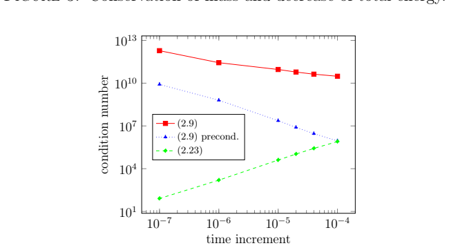
The load-bearing object is an explicit algebraic reduction of the coupled interior–boundary chemical-potential system. Starting from the monolithic system (2.15), the paper separates boundary and interior degrees of freedom, eliminates the interior chemical potential and the boundary chemical potential, and obtains a small symmetric positive definite boundary system with matrix $m L_\Omega|_{\Gamma\times\Gamma}+m_\Gamma M_\Omega|_{\Gamma\times\Gamma}M_\Gamma^{-1}L_\Gamma M_\Gamma^{-1}M_\Omega|_{\Gamma\times\Gamma}$. The resulting single nonlinear equation (2.23) for the new phase-field values has a structure that does not degenerate as $\tau\to0$, while still satisfying the compatibility constraint that makes it equivalent to the original coupled system. This reduction turns the numerical analysis into that of a standard Cahn–Hilliard scheme: a convex–concave splitting in time supplies unconditional energy stability, interpolation estimates supply the missing regularity, and a compactness argument identifies the limit.
What would settle it
For a manufactured smooth solution of (1.1) on a convex polygon with a polynomial double-well potential, take mesh and time-step pairs with $h^4/\tau\to 0$ and measure the discrete $L^2$ error; if the error does not tend to zero along such a sequence, the convergence claim of Theorem 4.4 is false.
Extended reading notes
Core claim
The paper's main result, Theorem 4.4, states that under assumptions on the mesh, the potentials, and the initial data, discrete solutions of scheme (2.9)/(2.23) converge along sequences $(h,\tau)\to 0$ to a triple $(\varphi,\mu,\mu_\Gamma)$ that solves the weak formulation (4.18) of the model. The potentials $F$ and $G$ must admit a convex–concave splitting with polynomial part of degree four plus a globally Lipschitz part; the initial data must have bounded energy; and the mesh and time step must satisfy $h^4/\tau\to0$ when the surface-diffusion coefficient $\kappa>0$, or $h^2/\tau\to0$ when $\kappa=0$. In the same framework the scheme conserves the phase-field mass in the domain and on the boundary separately, dissipates the discrete total energy, and has at least one solution for every time step. Passing to the limit in the scheme therefore also constitutes an existence proof for weak solutions.
Load-bearing premise
The convergence proof requires the mesh size $h$ and time step $\tau$ to satisfy $h^4/\tau\to0$ when $\kappa>0$ and $h^2/\tau\to0$ when $\kappa=0$; if a computation drives $\tau$ to zero on a fixed mesh, the bound on the discrete time derivative in the dual space is lost and the compactness argument that produces the weak solution no longer applies.
Editorial extensions
If this is right
- Discrete solutions exist for any time step size, without a CFL-type restriction, because the existence argument uses only the a priori energy estimate.
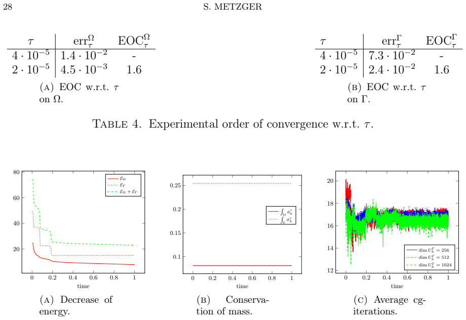
- The discrete total energy (bulk plus surface) decreases along solutions, and the mean phase-field values in the domain and on the boundary are conserved separately.
- Along mesh and time-step sequences satisfying condition (C), the discrete solutions yield weak solutions of the continuous model, so the scheme provides a constructive existence proof for the boundary-dynamics model.
- The same algebraic reduction and convergence analysis carry over to Allen–Cahn-type dynamic boundary conditions, including a dynamic contact-angle boundary condition.
- In the experiments, the phase field converges with experimental order about 2.3 with respect to mesh size in the bulk and 1.1 on the boundary, and order about 1.6 with respect to the time step.
Reading between the lines
- The refinement condition $h^4/\tau\to0$ (or $h^2/\tau\to0$ when $\kappa=0$) is a strong mesh–time coupling that adaptive time stepping may violate; testing convergence on fixed meshes as $\tau\to0$ would reveal whether this condition is an artifact of the proof.
- The boundary-only auxiliary system is symmetric positive definite, so in three dimensions the scheme's cost is dominated by a boundary problem; this suggests dedicated multilevel or preconditioned iterative solvers could make the method competitive for large-scale simulations.
- The same elimination strategy might extend to related bulk–surface phase-field models, such as models with non-instantaneous adsorption or reaction-rate transfer between boundary and bulk, wherever a compatibility relation between chemical potentials can be derived.
- The assumptions exclude singular potentials like logarithmic or double-obstacle wells; experimenting with penalized but smooth approximations may indicate whether the convergence theory can be pushed to singular potentials.
Signed reviews
Editorial analysis
A structured set of objections, weighed in public.
Referee Report
Summary. This paper proposes and analyzes a finite element scheme for the Cahn–Hilliard equation with dynamic boundary conditions of Liu–Wu type, where an additional Cahn–Hilliard equation on the boundary is coupled to the bulk equation through a normal-derivative term. The main contributions are: (i) an efficient reformulation of the fully discrete scheme that eliminates the two chemical potentials and avoids the degeneracy of the monolithic system as the time step tends to zero; (ii) a discrete energy-stability result (Lemma 3.3) and an existence result for discrete solutions (Lemma 3.4); (iii) a convergence theorem (Theorem 4.4) showing that discrete solutions converge along a sequence (h,τ)→0, under a mesh-time coupling condition, to a weak solution of the continuous model, thereby also providing an alternative existence proof; and (iv) numerical experiments documenting mass conservation, energy dissipation, conditioning behavior, and experimental orders of convergence.
Significance. If the results are correct, the paper gives a valuable toolbox for a nontrivial boundary-coupled Cahn–Hilliard system: an implementable, unconditionally energy-stable scheme whose convergence is proven, and a pathway to weak solutions that complements the gradient-flow existence theory of Garcke and Knopf. The paper is honest about its assumptions and provides detailed proofs for the main estimates, including the delicate interpolation-error control in Lemma 4.2. The simulations are reproducible in principle and illustrate the practical conditioning advantages of the proposed formulation. The main limitations are the restrictive mesh-time condition (C) in the convergence theorem and a few proof gaps that need to be closed before the claims are fully rigorous.
major comments (4)
- [§3, Lemma 3.4] The proof of Lemma 3.4 begins with "this allows us to assume w.l.o.g. that 1^T M_Ω Φ^n = 1^T M_Ω Φ^{n-1} = 0," but mass conservation alone does not justify a reduction to zero mean because the discrete scheme (2.23) is not invariant under adding a constant to Φ. The later inequality (3.13) uses the equivalence of sqrt(Φ^T L_Ω Φ) with the discrete L2 norm, which holds only on the mean-zero subspace. To make the argument rigorous for arbitrary initial data, the proof should work in the affine space of fixed total mass m_0, using a Poincaré-type inequality with the fixed mean, or should show that the energy estimate bounds the mean; otherwise the existence claim for general initial data is not established. This is a load-bearing step for the central existence result, although it is fixable.
- [§3, Lemma 3.4 statement] The statement of Lemma 3.4 lists only assumptions (T), (S1), (S2), and (P1), but the proof uses additional structure from (P2): the concavity inequality for G'_- with β, the polynomial-growth control of F'_-, and the discrete energy estimate of Lemma 3.3 that itself requires (P2). Either (P2) must be added to the lemma's hypotheses, or the proof must be modified to work under (P1) alone. As written, the statement and proof do not match.
- [§4, Assumption (C) and §5.1] Theorem 4.4 is conditional on the mesh-time coupling (C): h^4/τ→0 when κ>0 and h^2/τ→0 when κ=0. This is an explicit assumption, but it is strong: it requires τ to be much larger than h^4 (respectively h^2), so arbitrarily small time steps are admissible only on correspondingly fine meshes. The adaptive simulations in Section 5.1 use time increments down to 6.3·10^-7 on fixed or adaptively refined meshes, and the paper does not discuss how the adaptive time-stepping relates to condition (C). The authors should clarify that the convergence theorem applies to simultaneous refinement paths satisfying (C) and that the adaptive simulations in Section 5 are numerical demonstrations rather than instances covered by Theorem 4.4.
- [§4, Theorem 4.4, three-dimensional case] The passage to the limit in the nonlinear potential terms for d=3 is only sketched: the text says "The uniform bounds of φ_h^{τ,±} in L∞(0,T;H1(Ω)) provide enough regularity, to adapt the previously presented arguments to three spatial dimensions." For κ=0, the strong convergence (4.15f) on Γ holds only in L^s for s<4, while the cubic estimates (4.21)–(4.23) appear to require control in L^4(Γ). The exponent bookkeeping in three dimensions should be written out (or a precise embedding/interpolation argument given) so that the claimed validity of Theorem 4.4 for d=3 is fully supported.
minor comments (4)
- [§1, Eq. (1.16)] The definition of X_κ states "κ>1" in the first case and "κ=0" in the second, but the analysis throughout the paper treats all κ>0 as the surface-diffusion case. This appears to be a typo; it should read "κ>0".
- [Throughout] There are several typographical errors, including "asssume" in Section 2, "satifies" in Lemma 3.3, and the missing space in "tuple(φ,µ,µ Γ)" in Theorem 4.4. These should be corrected in a final revision.
- [§5.2, Table 3] The experimental order of convergence on Γ is 1.1, notably lower than the order 2.3 measured on Ω. The authors should comment on this discrepancy, since it may indicate a boundary-related suboptimality in the scheme or in the error measurement.
- [§4, Remark 4.5] Remark 4.5 claims that the convergence results carry over to Allen–Cahn-type boundary conditions, but it only lists the relevant uniform bounds and states that "we are able to identify converging subsequences and pass to the limit." Since this is an additional model with a different boundary equation, a brief sketch of the convergence argument (or a reference to the analogous steps) would be helpful.
Circularity Check
No circularity found: the scheme is a discretization of the continuous model and the convergence proof does not assume the target existence result.
full rationale
The derivation chain is self-contained. The discrete scheme (2.9) is obtained by applying mass-lumped finite elements and a convex-concave splitting directly to the weak form (1.15) of the continuous model (1.1), with the chemical potentials eliminated algebraically to obtain the implementable form (2.23); no parameter is fitted to data and no target quantity is used as an input. Stability (Lemma 3.3) and existence of discrete solutions (Lemma 3.4) are proved from the scheme itself. The convergence theorem (Theorem 4.4) uses only the a priori estimates of Corollary 4.1 and Lemma 4.2, together with compactness arguments, to extract subsequences and pass to the limit in (4.12), obtaining the weak formulation (4.18) without assuming that a continuous solution exists. The cited works are independent (e.g. Garcke and Knopf [26] for the generalized Poincare argument and uniqueness, and standard finite element references), and the author's self-citations concern implementation framework and adaptive mesh refinement, not the load-bearing convergence argument. The refinement condition (C) restricts the range of admissible (h,tau) pairs and is a stated hypothesis rather than a circular step; the adaptive simulations in Section 5 are not covered by Theorem 4.4, which is a limitation, not circularity. Accordingly no circular step is present.
Assumptions & free parameters
assumptions (5)
- domain assumption The potentials F and G admit convex-concave splittings satisfying (P1)-(P2), with polynomial part of degree four plus Lipschitz part; singular potentials (logarithmic, double obstacle) are excluded.
- domain assumption The spatial mesh is quasi-uniform and compatible on the boundary (S1)-(S2), and the domain is bounded, convex, and polygonal or polyhedral.
- domain assumption Initial data satisfy the uniform bound (I).
- domain assumption The refinement condition (C) holds: h^4/tau -> 0 for kappa>0 and h^2/tau -> 0 for kappa=0.
- standard math Brouwer fixed point theorem, Aubin-Lions lemma, Sobolev embeddings, Poincare inequalities, and standard finite element interpolation estimates are used as background.
Cite this review
Pith. "Pith review of An efficient and convergent finite element scheme for Cahn--Hilliard equations with dynamic boundary conditions." pith.science (2026). https://pith.science/paper/TZ5R566E
@misc{pith2026190804910,
  author       = {Pith},
  title        = {Pith review of: An efficient and convergent finite element scheme for Cahn--Hilliard equations with dynamic boundary conditions},
  year         = {2026},
  howpublished = {\url{https://pith.science/paper/TZ5R566E}},
  note         = {Machine review of arXiv:1908.04910}
}
read the original abstract
The Cahn--Hilliard equation is a widely used model that describes amongst others phase separation processes of binary mixtures or two-phase flows. In the recent years, different types of boundary conditions for the Cahn--Hilliard equation were proposed and analyzed. In this publication, we are concerned with the numerical treatment of a recent model which introduces an additional Cahn--Hilliard type equation on the boundary as closure for the Cahn--Hilliard equation in the domain [C. Liu, H. Wu, Arch. Ration. Mech. An., 2019]. By identifying a mapping between the phase-field parameter and the chemical potential inside of the domain, we are able to postulate an efficient, unconditionally energy stable finite element scheme. Furthermore, we establish the convergence of discrete solutions towards suitable weak solutions of the original model. This serves also as an additional pathway to establish existence of weak solutions. Furthermore, we present simulations underlining the practicality of the proposed scheme and investigate its experimental order of convergence.
Figures


Figures from the paper (6 more)




Forward citations
Cited by 1 Pith paper
-
Convergence of a Robin boundary approximation for a Cahn--Hilliard system with dynamic boundary conditions
Existence, uniqueness, and a linear-in-K error estimate are established for a Robin-boundary approximation of an extended Cahn-Hilliard system with affine dynamic boundary conditions.
Reference graph
Works this paper leans on
-
[1]
H. Abels and M. Wilke , Convergence to equilibrium for the Cahn–Hilliard equation with a log- arithmic free energy, Nonlinear Analysis: Theory, Methods & Applications, 67 (2007), pp. 3176 – 3193, https://doi.org/10.1016/j.na.2006.10.002
-
[2]
H. W. Alt , Linear functional analysis : An application-oriented introduction , Universitext„ Birkhäuser, London, 2016
work page 2016
-
[3]
J. W. Barrett, J. F. Blowey, and H. Garcke , Finite Element Approximation of the Cahn– Hilliard Equation with Degenerate Mobility, SIAM Journal on Numerical Analysis, 37 (1999), pp. 286– 318, https://doi.org/10.1137/s0036142997331669
-
[4]
J. W. Barrett, J. F. Blowey, and H. Garcke , On fully practical finite element approximations of degenerate Cahn-Hilliard systems, ESAIM: Mathematical Modelling and Numerical Analysis, 35 (2001), pp. 713–748,https://doi.org/10.1051/m2an:2001133
-
[5]
P. W. Bates and P. C. Fife , The Dynamics of Nucleation for the Cahn–Hilliard Equation, SIAM Journal on Applied Mathematics, 53 (1993), pp. 990–1008,https://doi.org/10.1137/0153049
-
[6]
J. F. Blowey, M. I. M. Copetti, and C. M. Elliott , Numerical analysis of a model for phase separation of a multi-component alloy, IMA Journal of Numerical Analysis, 16 (1996), pp. 111–139, https://doi.org/10.1093/imanum/16.1.111
-
[7]
J. F. Blowey and C. M. Elliott , The Cahn–Hilliard gradient theory for phase separation with non-smooth free energy Part I: Mathematical analysis, European Journal of Applied Mathematics, 2 (1991), pp. 233–280,https://doi.org/10.1017/s095679250000053x. 30 S. METZGER
-
[8]
J. F. Blowey and C. M. Elliott , The Cahn–Hilliard gradient theory for phase separation with non-smooth free energy Part II: Numerical analysis, European Journal of Applied Mathematics, 3 (1992), pp. 147–179,https://doi.org/10.1017/s0956792500000759
Show all 58 references
-
[9]
J. H. Bramble, J. E. Pasciak, and O. Steinbach , On the stability of theL2 projection inH 1(Ω), Math. Comp., 71 (2002), pp. 147–156,https://doi.org/S0025-5718(01)01314-X
2002
-
[10]
Brenner and L
S. Brenner and L. Scott , The Mathematical Theory of Finite Element Methods, Springer, 2002
2002
-
[11]
Campillo-Funollet, G
E. Campillo-Funollet, G. Grün, and F. Klingbeil , On modeling and simulation of electroki- netic phenomena in two-phase flow with general mass densities, SIAM Journal on Applied Mathe- matics, 72 (2012), pp. 1899–1925,https://doi.org/10.1137/120861333
2012 doi
-
[12]
Cheng, X
Q. Cheng, X. Yang, and J. Shen , Efficient and accurate numerical schemes for a hydro- dynamically coupled phase field diblock copolymer model, J. Comput. Phys., 341 (2017), pp. 44 – 60, https://doi.org/10.1016/j.jcp.2017.04.010
2017 doi
-
[13]
Cherfils, A
L. Cherfils, A. Miranville, and S. Zelik , The Cahn-Hilliard Equation with Logarithmic Potentials, Milan Journal of Mathematics, 79 (2011), pp. 561–596, https://doi.org/10.1007/ s00032-011-0165-4
2011
-
[14]
Chill, E
R. Chill, E. F ašangov á, and J. Prüss , Convergence to steady states of solutions of the Cahn–Hilliard and Caginalp equations with dynamic boundary conditions , Mathematische Nachrichten, 279 (2006), pp. 1448–1462,https://doi.org/10.1002/mana.200410431
2006 doi
-
[15]
Colli and T
P. Colli and T. Fukao , Cahn–Hilliard equation with dynamic boundary conditions and mass constraint on the boundary, JournalofMathematicalAnalysisandApplications, 429(2015), pp.1190– 1213, https://doi.org/10.1016/j.jmaa.2015.04.057
2015 doi
-
[16]
Colli, G
P. Colli, G. Gilardi, and J. Sprekels , On the Cahn–Hilliard equation with dynamic boundary conditions and a dominating boundary potential, Journal of Mathematical Analysis and Applications, 419 (2014), pp. 972–994,https://doi.org/10.1016/j.jmaa.2014.05.008
2014 doi
-
[17]
M. I. M. Copetti and C. M. Elliott , Numerical analysis of the Cahn–Hilliard equation with a logarithmic free Energy, Numer. Math., 63 (1992), pp. 39–65
1992
-
[18]
Elliott and H
C. Elliott and H. Garcke , On the Cahn–Hilliard Equation with Degenerate Mobility , SIAM Journal on Mathematical Analysis, 27 (1996), pp. 404–423, https://doi.org/10.1137/ S0036141094267662
1996
-
[19]
C. M. Elliott and A. M. Stuart , The Global Dynamics of Discrete Semilinear Parabolic Equa- tions, SIAM Journal on Numerical Analysis, 30 (1993), pp. 1622–1663,https://doi.org/10.1137/ 0730084
1993
-
[20]
C. M. Elliott and S. Zheng , On the Cahn–Hilliard equation, Archive for Rational Mechanics and Analysis, 96 (1986), pp. 339–357,https://doi.org/10.1007/BF00251803
1986 doi
-
[21]
H. P. Fischer, P. Maass, and W. Dieterich , Novel Surface Modes in Spinodal Decomposition, Physical Review Letters, 79 (1997), pp. 893–896,https://doi.org/10.1103/physrevlett.79.893
1997 doi
-
[22]
H. P. Fischer, P. Maass, and W. Dieterich , Diverging time and length scales of spinodal decomposition modes in thin films, Europhys. Lett., 42 (1998), pp. 49–54,https://doi.org/10. 1209/epl/i1998-00550-y
1998
-
[23]
Frank, A
F. Frank, A. Rupp, and D. Kuzmin , Bound-preserving flux limiting schemes for DG discretiza- tions of conservation laws with applications to the Cahn–Hilliard equation, Computer Methods in Ap- plied Mechanics and Engineering, 359 (2020), p. 112665,https://doi.org/10.1016/j.cma....
2020 doi
-
[24]
C. G. Gal, A Cahn–Hilliard model in bounded domains with permeable walls, Mathematical Methods in the Applied Sciences, 29 (2006), pp. 2009–2036,https://doi.org/10.1002/mma.757
2006 doi
-
[25]
Garcke, M
H. Garcke, M. Hinze, and C. Kahle , A stable and linear time discretization for a thermody- namically consistent model for two-phase incompressible flow, Applied Numerical Mathematics, 99 (2016), pp. 151 – 171,https://doi.org/10.1016/j.apnum.2015.09.002
2016 doi
-
[26]
Garcke and P
H. Garcke and P. Knopf , Weak Solutions of the Cahn–Hilliard System with Dynamic Boundary Conditions: A Gradient Flow Approach, SIAMJournalonMathematicalAnalysis, 52(2020), pp.340– 369, https://doi.org/10.1137/19M1258840
2020 doi
-
[27]
Gilardi, A
G. Gilardi, A. Miranville, and G. Schimperna , On the Cahn–Hilliard equation with irregular potentials and dynamic boundary conditions, Communications on Pure & Applied Analysis, 8 (2009), pp. 881–912,https://doi.org/10.3934/cpaa.2009.8.881. 31
2009 doi
-
[28]
G. R. Goldstein, A. Miranville, and G. Schimperna , A Cahn–Hilliard model in a domain with non-permeable walls, Physica D: Nonlinear Phenomena, 240 (2011), pp. 754–766,https://doi. org/10.1016/j.physd.2010.12.007
2011 doi
-
[29]
Grinfeld and A
M. Grinfeld and A. Novick-Cohen , Counting stationary solutions of the Cahn–Hilliard equation by transversality arguments, Proceedings of the Royal Society of Edinburgh: Section A Mathematics, 125 (1995), pp. 351–370,https://doi.org/10.1017/s0308210500028079
1995 doi
-
[30]
Grün, On convergent schemes for diffuse interface models for two-phase flow of incompressible fluids with general mass densities, SIAM J
G. Grün, On convergent schemes for diffuse interface models for two-phase flow of incompressible fluids with general mass densities, SIAM J. Numer. Anal., 51 (2013), pp. 3036–3061,https://doi. org/10.1137/130908208
2013 doi
-
[31]
G. Grün, F. Guillén-González, and S. Metzger , On fully decoupled, convergent schemes for diffuse interface models for two-phase flow with general mass densities, Commun. Comput. Phys., 19 (2016), pp. 1473–1502,https://doi.org/10.4208/cicp.scpde14.39s
2016 doi
-
[32]
Grün and F
G. Grün and F. Klingbeil , Two-phase flow with mass density contrast: stable schemes for a thermodynamic consistent and frame-indifferent diffuse-interface model, J. Comput. Phys., 257, Part A (2014), pp. 708–725,https://doi.org/10.1016/j.jcp.2013.10.028
2014 doi
-
[33]
Kenzler, F
R. Kenzler, F. Eurich, P. Maass, B. Rinn, J. Schropp, E. Bohl, and W. Dieterich , Phase separation in confined geometries: Solving the Cahn–Hilliard equation with generic boundary conditions, Computer Physics Communications, 133 (2001), pp. 139 – 157,https://doi.org/10. 1016/S0...
2001
-
[34]
Knopf, K
P. Knopf, K. F. Lam, C. Liu, and S. Metzger , Phase-field dynamics with transfer of materials: The Cahn–Hillard equation with reaction rate dependent dynamic boundary conditions, arXiv e-prints, (2020), http://arxiv.org/abs/2003.12983v1
2020 arXiv
-
[35]
Kufner, O
A. Kufner, O. John, and S. Fučík , Function spaces, Noordhoff, 1977
1977
-
[36]
Li and J
X. Li and J. Shen , On a SAV-MAC scheme for the Cahn-Hilliard-Navier-Stokes Phase Field Model, arXiv e-prints, (2019),https://arxiv.org/abs/1905.08504
2019 arXiv
-
[37]
Liero, Passing from bulk to bulk-surface evolution in the Allen–Cahn equation, Nonlinear Dif- ferential Equations and Applications NoDEA, 20 (2013), pp
M. Liero, Passing from bulk to bulk-surface evolution in the Allen–Cahn equation, Nonlinear Dif- ferential Equations and Applications NoDEA, 20 (2013), pp. 919–942,https://doi.org/10.1007/ s00030-012-0189-7
2013
-
[38]
Liu and H
C. Liu and H. Wu , An Energetic Variational Approach for the Cahn–Hilliard Equation with Dy- namic Boundary Condition: Model Derivation and Mathematical Analysis, Archive for Rational Me- chanics and Analysis, 233 (2019), pp. 167–247,https://doi.org/10.1007/s00205-019-01356-x,...
2019 doi
-
[39]
Metzger, On convergent schemes for two-phase flow of dilute polymeric solutions, ESAIM-MATH MODEL NUM, 52 (2018), pp
S. Metzger, On convergent schemes for two-phase flow of dilute polymeric solutions, ESAIM-MATH MODEL NUM, 52 (2018), pp. 2357–2408,https://doi.org/10.1051/m2an/2018042
2018
-
[40]
Metzger , On stable, dissipation reducing splitting schemes for two-phase flow of elec- trolyte solutions, Numerical Algorithms, 80 (2018), pp
S. Metzger , On stable, dissipation reducing splitting schemes for two-phase flow of elec- trolyte solutions, Numerical Algorithms, 80 (2018), pp. 1361–1390, https://doi.org/10.1007/ s11075-018-0530-2
2018
-
[41]
R. M. Mininni, A. Miranville, and S. Romanelli , Higher-order Cahn–Hilliard equations with dynamic boundary conditions, Journal of Mathematical Analysis and Applications, 449 (2017), pp. 1321–1339,https://doi.org/10.1016/j.jmaa.2016.12.071
2017 doi
-
[42]
Miranville and S
A. Miranville and S. Zelik , The Cahn–Hilliard equation with singular potentials and dynamic boundary conditions, Discrete & Continuous Dynamical Systems - A, 28 (2010), pp. 275–310,https: //doi.org/10.3934/dcds.2010.28.275
2010 doi
-
[43]
Motoda, Time periodic solutions of Cahn–Hilliard systems with dynamic boundaryconditions, AIMS Mathematics, 3 (2018), pp
T. Motoda, Time periodic solutions of Cahn–Hilliard systems with dynamic boundaryconditions, AIMS Mathematics, 3 (2018), pp. 263–287,https://doi.org/10.3934/math.2018.2.263
2018 doi
-
[44]
Nečas, Direct Methods in the Theory of Elliptic Equations, Springer Berlin Heidelberg, 2012, https://doi.org/10.1007/978-3-642-10455-8
J. Nečas, Direct Methods in the Theory of Elliptic Equations, Springer Berlin Heidelberg, 2012, https://doi.org/10.1007/978-3-642-10455-8
2012 doi
-
[45]
E. D. Nezza, G. Palatucci, and E. V aldinoci , Hitchhiker’s guide to the fractional Sobolev spaces, Bulletin des Sciences Mathématiques, 136 (2012), pp. 521–573,https://doi.org/https: //doi.org/10.1016/j.bulsci.2011.12.004
2012 doi
-
[46]
R. L. Pego , Front migration in the nonlinear Cahn–Hilliard equation, Proceedings of the Royal Society of London. A. Mathematical and Physical Sciences, 422 (1989), pp. 261–278,https://doi. org/10.1098/rspa.1989.0027. 32 S. METZGER
1989
-
[47]
T. Qian, X. W ang, and P. Sheng , A variational approach to the moving contact line hy- drodynamics, Journal of Fluid Mechanics, 564 (2006), pp. 333–360,https://doi.org/10.1017/ S0022112006001935
2006
-
[48]
Racke and S
R. Racke and S. Zheng , The Cahn–Hilliard equation with dynamic boundary conditions, Adv. Partial Differential Equations, 8 (2003), pp. 83–110
2003
-
[49]
Rybka and K.-H
P. Rybka and K.-H. Hoffmann , Convergence of solutions to Cahn–Hilliard equation, Commu- nications in Partial Differential Equations, 24 (1999), pp. 1055–1077,https://doi.org/10.1080/ 03605309908821458
1999
-
[50]
J. Shen, C. W ang, X. W ang, and S. Wise , Second-order Convex Splitting Schemes for Gradient Flows with Ehrlich–Schwoebel Type Energy: Application to Thin Film Epitaxy, SIAM J. Numer. Anal., 50 (2012), pp. 105–125,https://doi.org/10.1137/110822839
2012 doi
-
[51]
Shen and X
J. Shen and X. Yang , Numerical approximations of Allen-Cahn and Cahn-Hilliard equations, Dis- crete Cont. Dyn. S., 28 (2010), pp. 1669–1691,https://doi.org/10.3934/dcds.2010.28.1669
2010 doi
-
[52]
P. A. Thompson and M. O. Robbins , Simulations of contact-line motion: Slip and the dy- namic contact angle, Physical Review Letters, 63 (1989), pp. 766–769,https://doi.org/10.1103/ physrevlett.63.766
1989
-
[53]
Trautwein, Finite-Elemente Approximation der Cahn–Hilliard-Gleichung mit Neumann- und dynamischen Randbedingungen
D. Trautwein, Finite-Elemente Approximation der Cahn–Hilliard-Gleichung mit Neumann- und dynamischen Randbedingungen. Bachelor thesis, University of Regensburg, 2018
2018
-
[54]
S. Wise, C. W ang, and J. Lowengrub , An Energy-Stable and Convergent Finite-Difference Scheme for the Phase Field Crystal Equation, SIAM J. Numer. Anal., 47 (2009), pp. 2269–2288, https://doi.org/10.1137/080738143
2009 doi
-
[55]
Wu and S
H. Wu and S. Zheng , Convergence to equilibrium for the Cahn–Hilliard equation with dynamic boundary conditions, Journal of Differential Equations, 204 (2004), pp. 511–531,https://doi.org/ 10.1016/j.jde.2004.05.004
2004 doi
-
[56]
Xu and T
C. Xu and T. Tang , Stability Analysis of Large Time-Stepping Methods for Epitaxial Growth Models, SIAM J. Numer. Anal., 44 (2006), pp. 1759–1779,https://doi.org/10.1137/050628143
2006 doi
-
[57]
Yang and G
X. Yang and G. Zhang , Numerical approximations of the Cahn-Hilliard and Allen-Cahn Equations with general nonlinear potential using the Invariant Energy Quadratization approach, arXiv e-prints, (2015), https://arxiv.org/abs/1712.02760
2015 arXiv
-
[58]
Zheng , Asymptotic behavior of solution to the Cahn–Hillard equation, Applicable Analysis, 23 (1986), pp
S. Zheng , Asymptotic behavior of solution to the Cahn–Hillard equation, Applicable Analysis, 23 (1986), pp. 165–184,https://doi.org/10.1080/00036818608839639
1986 doi
Reviewed August 14, 2026 · model on record in the stance chip above.
Discussion (0). Continue with ORCID to comment.