REVIEW 2 major objections 5 minor 44 references
Reconstructing compound objects by quantum imaging with higher-order correlation functions
T0 review · 2 major / 5 minor · reviewed 2026-08-14 · deepseek-v4-flash
Pith's one-line read Parametric locality, visible as band structure in the Fisher information matrix, enables a sliding-window estimator that reconstructs super-resolved quantum images at linear cost and predicts the optimal photon correlation width.
desk verdict A solid, useful paper whose main algorithmic claim is real but whose linear-complexity statement is oversold in the super-resolution regime. read the letter →
The pith
A machine-rendered reading of the paper's core claim, the machinery that carries it, and where it could break.
The reading
What carries the argument
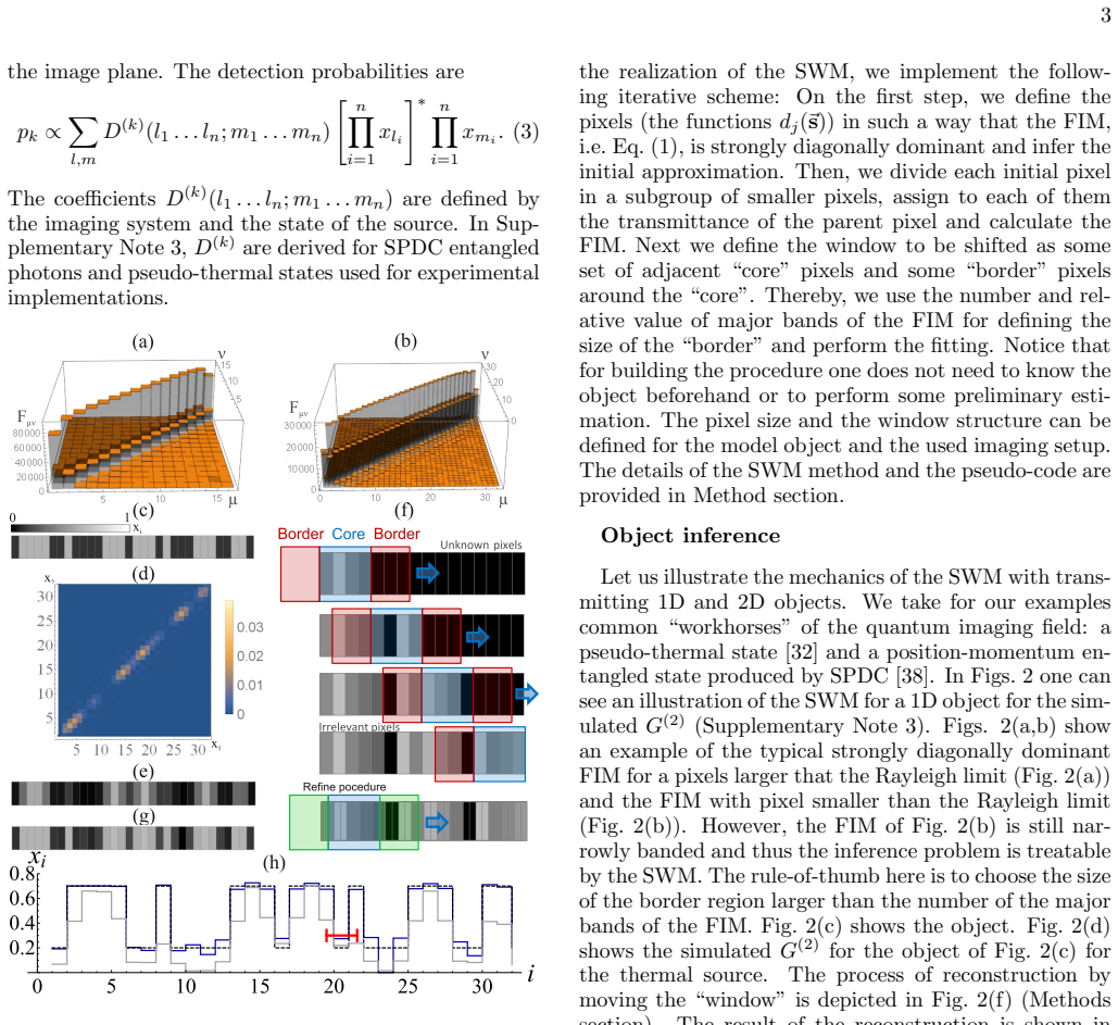
The central object is the Fisher information matrix of a parametrically l-local measurement, where each outcome probability has nonzero derivatives only with respect to parameters within distance l, so the matrix is l-banded. The argument uses the matrix fact that inverses of banded matrices are approximately banded, which turns the error bound for one parameter into a function of nearby parameters only. The sliding window method is the estimator built from that fact: after a coarse first pass with pixels large enough for diagonal dominance, it refines the grid and, in each step, fits only a core window of unknown pixels surrounded by a border whose width exceeds the number of major Fisher information bands; values outside the window are held fixed or set to zero. The border width, not the total number of pixels, sets the cost of every local fit, and shifting the core window across the object produces the claimed linear total complexity.
What would settle it
Calculate the number of significant Fisher information bands, n0 = Δl/d, for a one-dimensional near-field image on grids with d = Δl/2, Δl/4, and Δl/8. If the required border size grows with n0 rather than remaining bounded, the per-window cost grows with the number of pixels and the linear-complexity claim is refuted; the paper reports no benchmark of this scaling.
Extended reading notes
Core claim
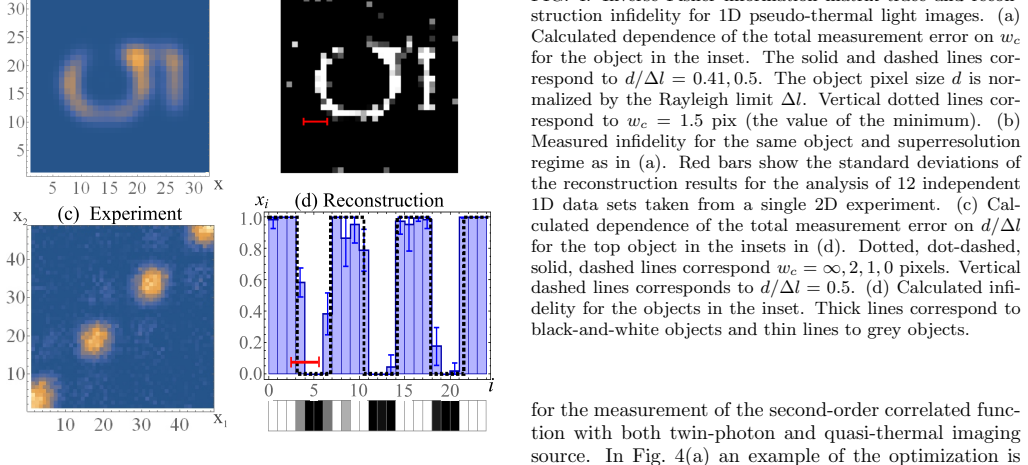
The paper's central discovery is that the hard nonlinear estimation problem of quantum imaging becomes tractable when the measurement is parametrically local: when each detected correlation event depends on a small cluster of nearby pixels, the Fisher information matrix is narrowly banded, and the standard lower bound on estimator variance for a given pixel depends only on data in a window around it. The authors build the sliding window method on this: first a coarse reconstruction with large pixels whose Fisher information matrix is diagonally dominant, then refinement on a finer pixel grid where each optimization step treats a core of unknown pixels, a border of known or ignored pixels, and a border size set by the number of major Fisher information bands. They demonstrate the method on simulated and experimental data, reconstructing grey transmission objects from measured second- and third-order correlation functions for pseudo-thermal light and for position-momentum entangled twin photons, and report resolution beyond the Rayleigh limit. The paper also establishes two further results from the same information analysis: an optimal correlation width of the imaging field, approximately the size of the smallest object detail, and an improvement of resolution from the estimation bias that arises when parameters sit at the boundary of their allowed range.
Load-bearing premise
The load-bearing premise is that the measurement is parametrically local at the finest pixel grid used: the width of the Fisher information bands stays small relative to the total number of parameters as the grid is refined below the Rayleigh limit, so a fixed-size window border can keep the local fits accurate.
Editorial extensions
If this is right
- For objects with many pixels, each reconstruction step becomes a small least-squares fit over a window, so the total computational cost scales linearly with the number of parameters instead of with a high power of it.
- In the super-resolution regime, the best photon-source correlation width is not the smallest possible but roughly the smallest object feature size, giving a design rule for choosing source speckle size or twin-photon correlation width.
- Higher-order correlation measurements with both pseudo-thermal and entangled twin-photon sources can reconstruct grey transmission objects beyond the Rayleigh limit.
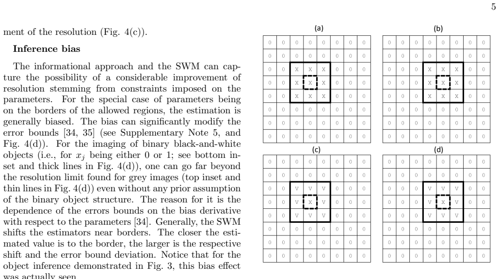
- When estimated parameters lie at the boundary of their allowed range, the resulting estimate bias can lower the total reconstruction error, so binary objects can be resolved better than the unbiased error bound suggests.
- The Fisher-information analysis can be performed per imaging setup without knowing the object, so the window structure and border size can be fixed in advance from the point-spread function and source correlations.
Reading between the lines
- The same windowing principle should carry over to any nonlinear estimation problem whose Fisher information matrix is banded, not only optical imaging; the argument never uses the specific imaging model except to establish locality.
- A direct stress test is to benchmark how the required border size grows as the pixel grid is refined below the Rayleigh limit; the linear-complexity claim assumes this growth stays bounded while the number of parameters increases.
- The reported resolution gain from boundary bias suggests that encoding object constraints, such as known binary or grey-value bounds, is not just a prior but a measurable information resource worth quantifying separately from the correlation statistics.
- One could test the optimal-correlation-width rule by measuring reconstruction infidelity versus source correlation width across several feature sizes and checking whether the minimum tracks the feature size, as the paper reports for one object.
Signed reviews
Editorial analysis
A structured set of objections, weighed in public.
Referee Report
Summary. The manuscript proposes an iterative sliding-window method (SWM) for nonlinear parameter estimation in problems with parametrically local measurements, i.e., measurements where each observed probability depends on a limited subset of the unknown parameters. The authors connect this locality to the banded structure of the Fisher information matrix (FIM), use the FIM to choose the window and border sizes, and apply the method to near-field quantum imaging with higher-order correlation functions. They derive the relevant detection coefficients for pseudo-thermal and SPDC sources, demonstrate reconstructions on simulated and experimental data, predict an optimal source correlation width from the trace of the inverse FIM, and experimentally confirm the prediction. They additionally discuss how estimation bias arising from parameter constraints can improve resolution.
Significance. If the linear-complexity claim is sustained, the SWM is a potentially valuable tool for quantum imaging and tomography with large parameter spaces. The paper has several concrete strengths: the FIM-based locality analysis is clearly presented, the pseudo-code is implementable, and the experimental demonstrations with a 32x32 SPAD array for both pseudo-thermal and SPDC sources are credible. The prediction of an optimal correlation width from the Fisher-information model and its confirmation with experimental reconstruction infidelity (Fig. 4a,b) is a nontrivial, falsifiable result. The biased-estimation discussion correctly draws on the constrained-estimation literature. However, the central scaling claim is not rigorously established for the super-resolution regime, and the window-truncation approximation lacks an error bound; these issues need to be addressed before the claimed complexity advantage can be accepted.
major comments (2)
- [Abstract; Results (Theoretical background); Methods (Sliding windows method)] The central complexity claim, stated in the abstract as 'this iterative scheme is linear on the total number of parameters,' is not established for the super-resolution regime in which the method is applied. In Supplementary Note 3, n0 = Delta_l / d is the width of the point-spread function in object-pixel units. For a fixed physical object, refining the pixel grid below the Rayleigh limit makes the total pixel count M grow while n0 grows proportionally to M. The Methods pseudo-code sizes the window border from the 'number and relative value of major bands of the FIM,' so each local minimization at a given shift involves O(n0) unknown and known pixels, and the number of shifts is only O(M/n0). The total cost is therefore O(M) only under the unstated assumption that n0 remains O(1) as the grid is refined. Since the experiments use a fixed 32x32 detector array, they do not exercise the scaling regime in which the problem is claimed to become hard. Please state the assumptions under which the claimed linearity holds, or qualify the claim in the abstract and introduction.
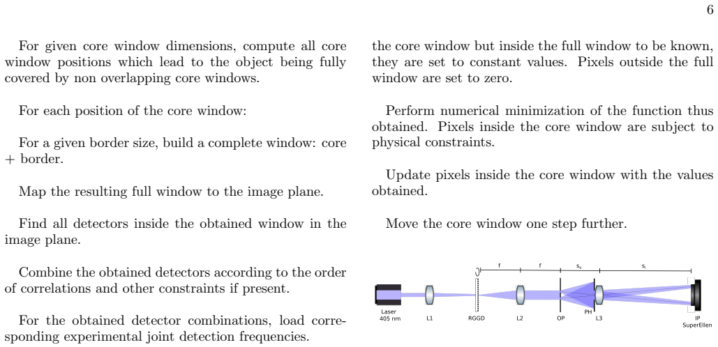
- [Methods (pseudo-code, first approximation and refinement)] The truncation approximation used in both algorithms is stated as 'the theoretical probabilities are computed assuming all pixels but those inside the window to be zero' (first approximation) and 'pixels outside the full window are set to zero' (refinement), but no error bound is given for this approximation. The size of the omitted-pixel contribution is controlled by the same PSF tails that define n0; when d is reduced toward the super-resolution regime, n0 grows and the number of omitted pixels with non-negligible weight grows as well, so the bias introduced by the truncation is not controlled. A quantitative error bound, or at least a numerical convergence check as a function of the window and border sizes, is needed to justify the accuracy of the SWM reconstructions in the claimed regime.
minor comments (5)
- [Supplementary Note 3, paragraph after Eq. (22)] The sentence stating that the coefficients are 'effectively zero for |j-m| << n0 or |k-n| << n0' appears to have the inequality reversed: if n0 is the PSF width in object pixels, the coefficients should be negligible for separations much larger than n0, not much smaller. Please correct this.
- [Supplementary Note 4] The text refers to 'the Appendix C' for the spatial correlation function, but the manuscript contains no Appendix C; the relevant description appears in Supplementary Note 3. Please update the cross-reference.
- [Results (Experiment); Fig. 3] The claim of resolution beyond the Rayleigh limit is supported visually by the red bars in Fig. 3, but a quantitative definition of achieved resolution (for example, estimated feature widths with uncertainties derived from the FIM or from repeated reconstructions) would make the claim more precise and easier to evaluate.
- [Data availability] The statement 'The code itself is available upon request' is weaker than the rest of the reproducibility effort; depositing the code in a permanent repository would allow readers to reproduce the reconstructions and the linear-complexity experiments.
- [Results (Theoretical background)] The definition of strict parametric l-locality is given for a one-dimensional ordering of parameters, while the imaging demonstrations are two-dimensional. Please state how the locality condition and the window construction generalize to two dimensions (for example, using a Chebyshev or Euclidean distance between pixel indices).
Circularity Check
No circular derivation: the central claims are model-based predictions tested against known USAF benchmarks; self-citations are non-load-bearing.
full rationale
The paper's central derivation is self-contained. The SWM is constructed from the banded structure of the FIM, with locality derived from the PSF and source correlation functions (Supplementary Note 3, Eqs. (16)-(22)); the linear-complexity statement is an algorithmic property of the sliding-window iteration, not a quantity fitted from the data. The optimal-correlation-width prediction is computed from the trace of the inverse FIM (Fig. 4(a), Supplementary Note 4) and then tested against reconstruction infidelity for known USAF targets (Fig. 4(b)), so the predicted quantity is not used as an input to the reconstruction in a way that forces the claimed agreement. The only self-citations are to the detector characterization [36,37] and to data-pattern tomography as an example of parametric locality [15]; neither is load-bearing for the paper's central inference claims. The scaling concern about the window border growing with n0 = Delta_l/d is a correctness risk about the complexity claim in the deep super-resolution limit, not a circularity.
Assumptions & free parameters
free parameters (3)
- Window border/core sizes =
Rule of thumb: border larger than the number of major FIM bands; no precise numeric value given
- Source correlation width wc =
Varied; optimum at wc = 1.5 pix in Fig. 4(a), measured via Gaussian fit to G(2)
- Initial pixel size d_initial =
Chosen so the inverse FIM is diagonally dominant
assumptions (7)
- standard math Inverses of banded matrices can be approximated by banded matrices (Refs [21,22])
- standard math Fisher information matrix Eq. (1) and Cramér-Rao bound Eq. (9), plus biased CRB Eq. (28) from Eldar [34,35]
- domain assumption Pseudo-thermal source has Gaussian statistics and nth-order correlations factor into pairwise products (Eq. 16, Supp Note 3)
- domain assumption SPDC joint-position amplitude is approximately a Gaussian function with width wc (Supp Note 3)
- domain assumption Near-field PSF is a jinc function with phase factor approximately 1, and coefficients D vanish for |j-m| >> n0 = Δl/d (Supp Note 3)
- ad hoc to paper In the first approximation, pixels outside the full window are set to zero; in refinement, pixels outside the core but inside the full window are treated as known constants (Methods pseudocode)
- ad hoc to paper Border size is chosen larger than the number of major FIM bands, with no rigorous guarantee of sufficient accuracy
Cite this review
Pith. "Pith review of Reconstructing compound objects by quantum imaging with higher-order correlation functions." pith.science (2026). https://pith.science/paper/U4V63XU6
@misc{pith2026190807461,
  author       = {Pith},
  title        = {Pith review of: Reconstructing compound objects by quantum imaging with higher-order correlation functions},
  year         = {2026},
  howpublished = {\url{https://pith.science/paper/U4V63XU6}},
  note         = {Machine review of arXiv:1908.07461}
}
read the original abstract
Quantum imaging has a potential of enhancing precision of the object reconstruction by using quantum correlations of the imaging field. This is especially important for imaging requiring low-intensity fields up to the level of few-photons. However, quantum imaging generally leads to nonlinear estimation problems. The complexity of these problems rapidly increases with the number of parameters describing the object. We suggest a way to drastically reduce the complexity for a wide class of problems. The key point of our approach is connecting the features of the Fisher information with the parametric locality of the problem, and building the efficient iterative inference scheme reconstructing only a subset of the whole set of parameters in each step. This iterative scheme is linear on the total number of parameters. This scheme is applied to quantum near-field imaging, the inference procedure is developed resulting in super-resolving reconstruction of grey compound transmission objects. The functionality of the method is demonstrated with experimental data obtained by measurements of higher-order correlation functions for imaging with entangled twin-photons and pseudo-thermal light sources. By analyzing the informational content of the measurement, it becomes possible to predict the existence of optimal photon correlations providing for the best image resolution in the super-resolution regime. This prediction is experimentally confirmed. It is also shown how an estimation bias stemming from image features may drastically improve the resolution.
Figures


Figures from the paper (8 more)



Reference graph
Works this paper leans on
-
[1]
E. J. Candes, J. K. Romberg, and T. Tao, IEEE Trans. Inform. Theory 52, 489509 (2006)
work page 2006
-
[2]
D. L. Donoho, IEEE Trans. Inform. Theory 52, 12891306 (2006)
work page 2006
-
[3]
D. Gross, Yi-Kai Liu, S. T. Flammia, S. Becker, and J. Eisert, Phys. Rev. Lett. 105, 150401 (2010)
work page 2010
-
[4]
C. A. Riofrio, D. Gross, S. T. Flammia, T. Monz, D. Nigg, R. Blatt and J. Eisert, Nat. Comm. 8, 15305 (2017)
work page 2017
- [5]
- [6]
-
[7]
T. Moroder, P. Hyllus, G. T´ oth, C. Schwemmer, A. Niggebaum, S. Gaile, O. G¨ uhne, and H. Weinfurter, New J. Phys. 14, 105001 (2012)
work page 2012
-
[8]
C. Schwemmer, G. T´ oth, A. Niggebaum, T. Moroder, D. Gross, O. G¨ uhne, and H. Weinfurter, Phys. Rev. Lett. 113, 040503 (2014)
work page 2014
Show all 44 references
-
[9]
Thiebaut, J
E. Thiebaut, J. Young, JOSA A 34 904 (2017)
2017
-
[10]
J. M. Ortega and W. C. Rheinboldt, Iterative Solution of Nonlinear Equations in Several Variables (Academic Press Inc, San Diego, 1970)
1970
-
[11]
H. R. Haffner, W. Hansel, C. F. Roos, J. Benhelm, D. Chek-al-kar, M. Chwalla, T. Korber, U. D. Rapol, M. Riebe, P. O. Schmidt, C. Becher, O. Ghne, W. Dur & R. Blatt, Nature 438, 643 (2005)
2005
-
[12]
Bloch, J
I. Bloch, J. Dalibard, & W. Zwerger, Rev. Mod. Phys. 80, 885 (2008)
2008
-
[13]
Tetienne, N
J.-Ph. Tetienne, N. Dontschuk, D. A. Broadway, A. Stacey, D. A. Simpson, and L. C. L. Hollenberg, Sci. Adv. 3, e1602429 (2017)
2017
-
[14]
Shih, IEEE Journal of Selected Topics in Quantum Electronics, IEEE 13, 1016 (2007)
See, for example, Y.H. Shih, IEEE Journal of Selected Topics in Quantum Electronics, IEEE 13, 1016 (2007)
2007
-
[15]
Rehacek, D
J. Rehacek, D. Mogilevtsev, and Z. Hradil, Phys. Rev. Lett. 105, 010402 (2010)
2010
-
[16]
Tsang, R
M. Tsang, R. Nair, and X.-M. Lu, Phys. Rev. X6, 031033 (2016). 8
2016
-
[17]
Nair and M
R. Nair and M. Tsang, Phys. Rev. Lett. 117, 190801 (2016)
2016
-
[18]
Motka, B
L. Motka, B. Stoklasa, M. DAngelo, P. Facchi, A. Garuc- cio, Z. Hradil, S. Pascazio, F.V. Pepe, Y.S. Teo, J. Re- hacek, L.L. Sanchez-Soto, The European Physical Jour- nal Plus, 131, 130 (2016)
2016
-
[19]
Rehacek, Z
J. Rehacek, Z. Hradil, B. Stoklasa, M. Paur, J. Grover, A. Krzic, L.L. Sanchez-Soto, Phys. Rev. A 96 062107 (2017)
2017
-
[20]
Seveso, M
L. Seveso, M. A. C. Rossi, and M. G. A. Paris, Phys. Rev. A 95, 012111 (2017)
2017
-
[21]
Bickel and M
P. Bickel and M. Lindner, Theory Probab. Appl. 56, 1 (2012)
2012
-
[22]
Demko, W
S. Demko, W. F. Moss, and P. W. Smith, Math. Comp., 43 491 (1984)
1984
-
[23]
Born and E
M. Born and E. Wolf, Principles of Optics (Cambridge University Press, Cambridge, UK, 1999)
1999
-
[24]
Zhang, W
P. Zhang, W. Gong, Xia Shen, D. Huang, and S. Han, Opt. Lett. 34, 1222 (2009)
2009
-
[25]
Chen, I.N
X.-H. Chen, I.N. Agafonov, K.-H. Luo, Q. Liu, R. Xian, M.V.Chekhova, and L.-A. Wu, Opt. Lett. 53, 1166 (2010)
2010
-
[26]
Y. Zhou, J. Simon, J. Liu, and Y. Shih, Phys. Rev. A 81, 043831 (2010)
2010
-
[27]
Gatto Monticone, K
D. Gatto Monticone, K. Katamadze, P. Traina, E. Moreva, J. Forneris, I. Ruo-Berchera, P. Olivero, I.P. De- giovanni, G. Brida, and M. Genovese, Phys. Rev. Lett. 113, 143602 (2014)
2014
-
[28]
Israel, R
Y. Israel, R. Tenne, D. Oron and Y. Silberberg, Nat. Comm. 8, 14786 (2017)
2017
-
[29]
Tenne, U
R. Tenne, U. Rossman, B. Rephael, Y. Israel, A. Krupinski-Ptaszek, R. Lapkiewicz, Y. Silberberg and D. Oron, Nat. Phot. 13, 116 (2019)
2019
-
[30]
Classen, F
A. Classen, F. Waldmann, S. Giebel, R. Schneider, D. Bhatti, Th. Mehringer, and J. von Zanthier, Phys. Rev. Lett. 117, 253601 (2016)
2016
-
[31]
Classen, J
A. Classen, J. von Zanthier, M. O. Scully, and G. S. Agarwal, Optica 4, 580 (2017)
2017
-
[32]
Martienssen and E
W. Martienssen and E. Spiller, Am. J. Phys. 32(12), 919 (1964)
1964
-
[33]
Statistical properties of laser speckle patterns
J. W. Goodman, “Statistical properties of laser speckle patterns”, in Laser speckle and related phenomena , vol. 9 of Toppics in Applied Physics, J. C. Dainty, ed., (Springer, Berlin, 1975)
1975
-
[34]
Y. C. Eldar, Foundations and Trends in Signal Process- ing, 1 305 (2008)
2008
-
[35]
Y. C. Eldar, IEEE Trans. Signal Processing, 52, 1916 (2004)
2004
-
[36]
Gasparini, M
L. Gasparini, M. Zarghami, H. Xu, L. Parmesan, M. M. Garcia, M. Unternhrer, B. Bessire, A. Stefanov, D. Stoppa, and M. Perenzoni, “A 32 ×32-pixels time- resolved singlephoton image sensor with 44.64- µm pitch and 19.48% fill-factor with on-chip row/frame skipping features reach...
2018
-
[37]
Unternahrer, B
M. Unternahrer, B. Bessire, L. Gasparini, M. Perenzoni, and A. Stefanov, Optica 5(9), 1150–1154 (2018)
2018
-
[38]
S. P. Walborn, C. H. Monken, S. Padua, and P. H. Ribeiro, Physics Reports 495, 87–139 (2010)
2010
-
[39]
Liu, T.Z
X.Q. Liu, T.Z. Huang and Y.D. Fu, Appl. Math. Lett., 19 590 (2006)
2006
-
[40]
Politi, M
T. Politi, M. Popolizio, JIPAM 9, 31 (2008)
2008
-
[41]
Zhuohong Huang, Jianzhou Liu, Applied Mathematics E-Notes, 10, 11-18 (2010)
2010
-
[42]
WoIkowicz, G
H. WoIkowicz, G. P. H. Styan, Linear Algebra and its Applications 29, 471 (1980)
1980
-
[43]
Emanueli, and A
S. Emanueli, and A. Arie, Appl. Opt. 42, 6661 (2003)
2003
-
[44]
Schneeloch, and J
J. Schneeloch, and J. C. Howell, J. Opt. 18, 053501 (2016) Supplementary note 1. Bounds for inverses of banded and approximately banded matrices Here we give a number of known results about inverses of banded and approximately banded matrices useful for our discussion. First o...
2016
Reviewed August 14, 2026 · model on record in the stance chip above.
Discussion (0). Continue with ORCID to comment.