REVIEW 4 major objections 5 minor 28 references
Faster Computation of Entropic Optimal Transport via Stable Low Frequency Modes
T0 review · 4 major / 5 minor · reviewed 2026-08-07 · deepseek-v4-flash
Pith's one-line read SK–NR(ℓ) accelerates Sinkhorn by restricting Newton–Raphson steps to the ℓ low-frequency modes that cause the small-ε slowdown.
desk verdict Nice structural result and a clever algorithm, but the complexity analysis is wrong as written, so the wall-clock speedups are unverified. read the letter →
The pith
A machine-rendered reading of the paper's core claim, the machinery that carries it, and where it could break.
The reading
What carries the argument
The central object is the operator $K_\varepsilon$ on $H = L^2(X;\alpha) \oplus L^2(Y;\beta)$, defined by $K_\varepsilon(f_1 \oplus g_1) = \mathrm{Op}(\pi^*_\varepsilon)(g_1) \oplus \mathrm{Op}(\pi^*_\varepsilon)^T(f_1)$, where the Gibbs kernel $\exp((f^*(x)+g^*(y)-C(x,y))/\varepsilon)$ integrates against $\beta$ or $\alpha$. In block form $K_\varepsilon = \begin{pmatrix} 0 & R \\ R^T & 0 \end{pmatrix}$, so its spectrum is the set of signed singular values of $R$, and Perron–Frobenius theory places the spectrum in $[-1, 1]$; the constant direction is the unique eigenvalue-$1$ eigenvector. The structure theorem $\nabla^2 Q_\varepsilon(f^*,g^*) = -\frac{1}{\varepsilon}(\mathrm{Id}_H + K_\varepsilon)$ makes $K_\varepsilon$ the Hessian of the dual, while Lemma 3.2 makes it the linearization of the Sinkhorn iteration, so one spectral object explains both the slow fixed-point convergence and the ill-conditioning that any second-order method must fix. The algorithm's Newton step is the projected Newton–Raphson step for the semi-dual objective $Q^{\mathrm{semi}}_\varepsilon$, whose Hessian at $f^*$ equals $-\frac{1}{\varepsilon}(\mathrm{Id} - RR^T)$, so the eigen-information needed for the dual and semi-dual formulations is equivalent.
What would settle it
Compute the exact top-ℓ eigenspace of $\nabla^2 Q^{\mathrm{semi}}_\varepsilon(f^*)$ for a fixed problem at a sequence of ε values, and measure the operator norm $\|\Pi_{V_\ell(\varepsilon)} - \Pi_{V_\ell(\varepsilon')}\|_{\mathrm{op}}$ between the projector at the target ε and the projector at the warm-start $\varepsilon'$. If this norm does not go to 0 as $\varepsilon' \to \varepsilon$, or if it is large for the $\varepsilon'$ values used in the paper's protocol, then the error estimate of Theorem 4.2 with $V_\ell = V_\ell(\varepsilon)$ does not apply, and the observed acceleration would be due to something other than the claimed contraction-rate mechanism.
Extended reading notes
Core claim
At the optimal Kantorovich potentials, the Hessian of the EOT dual objective factorizes as $\nabla^2 Q_\varepsilon(f^*, g^*) = -\frac{1}{\varepsilon}(\mathrm{Id}_H + K_\varepsilon)$, where $K_\varepsilon$ is a self-adjoint integral operator with spectrum in $[-1, 1]$, symmetric about zero, and with a spectral gap. The same operator is the linearization of the Sinkhorn fixed-point map, so the directions that make the dual Hessian nearly singular are exactly the directions along which Sinkhorn contracts most slowly. The paper's algorithm SK–NR(ℓ) computes ℓ low-frequency eigenvectors once at a larger regularization $\varepsilon'$ (a spectral warm-start) and then interleaves standard Sinkhorn rescaling with Newton–Raphson steps on the span of those vectors. Theorem 4.2 proves the iteration error satisfies $\|f_{k+1} - f^*\| \le \rho_{\ell+1}^2 \|f_k - f^*\| + C\|f_k - f^*\|^2$ when $V_\ell$ is the exact eigenspace of $\nabla^2 Q^{\mathrm{semi}}_\varepsilon$, so the linear contraction is set by the $(\ell+1)$-st eigenvalue of $K_\varepsilon$ instead of $\rho_1$. Because $\rho_{\ell+1}$ is closer to the spectrally stable interior, the iteration count shrinks exponentially with each additional Newton direction as $\varepsilon \to 0$; this is the mechanism behind the order-of-magnitude speed-ups reported on Gaussian and single-cell tasks.
Load-bearing premise
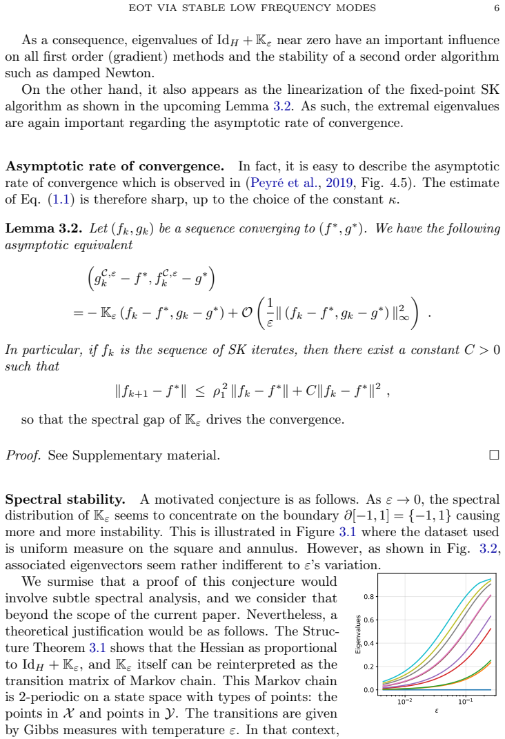
The accelerated rate is proved under the assumption that the few directions used for the Newton step are exactly the unstable directions at the target regularization; the algorithm instead computes them once at a larger regularization and the paper relies on an unproved conjecture that these directions stay almost the same as the regularization is lowered. If that conjecture fails, the promised faster contraction rate is not guaranteed.
Editorial extensions
If this is right
- With $V_\ell$ spanned by the ℓ leading eigenvectors, SK–NR(ℓ) contracts at rate $\rho_{\ell+1}^2$ rather than $\rho_1^2$, replacing the bad small-ε exponent $\lambda_1$ by $\lambda_{\ell+1}$ in the iteration-count asymptotics $N \asymp \exp(\lambda_{\ell+1}/\varepsilon) \log(1/\omega)$.
- Per-iteration cost stays $O(nm + \ell^3)$, so for $\ell \ll (nm)^{1/3}$ the overhead is negligible and the acceleration is essentially free in wall-clock time; the reported experiments show nearly identical per-iteration cost.
- Because the smallest eigenvectors of $K_\varepsilon$ can be recovered from the largest via the symmetry $u \oplus v \leftrightarrow (-u) \oplus v$, only a partial power-method eigensolve of scale ℓ is needed, not a full spectral decomposition.
- The global convergence proof only requires the extra step to increase $Q^{\mathrm{semi}}_\varepsilon$, so the spectral/Newton correction can be replaced by any other ascent direction; the projection onto ℓ unstable directions is the version that maximises the gain per low-dimensional solve.
- For small ε, the empirical gains on the single-cell task show that with a modest ℓ = 30, the method reaches a given marginal-error tolerance in a small fraction of the vanilla Sinkhorn iterations, bringing trajectory-inference-scale problems closer to practical runtime.
Reading between the lines
- A direct check the authors leave open: measure $\|\Pi_{V_\ell(\varepsilon)} - \Pi_{V_\ell(\varepsilon')}\|_{\mathrm{op}}$ on standard cost families (squared Euclidean, ground metric) to see for which $\varepsilon'/\varepsilon$ ratios the warm-started projector stays within the regime where the $\rho_{\ell+1}^2$ bound applies. If the norm grows with the geometry of the marginals, the practical rule
- The 2-periodic Markov-chain reading of $K_\varepsilon$ suggests that spectral-clustering heuristics (nodal domains of the Gibbs kernel, Cheeger-type ratios) could predict which directions are the unstable low-frequency ones, making the method applicable before computing any eigenvectors.
- The Hessian identity could support an adaptive version of the algorithm that monitors the top singular values of $R$ during the Sinkhorn run and increases ℓ only when $\rho_{\ell+1}^2$ is not small enough, instead of fixing ℓ in advance.
- Because Newton's step is only on ℓ coordinates, implicit differentiation of the fixed point could restore differentiability through SK–NR(ℓ), which the paper notes is lost in the forward loop; that would let the accelerated solver plug into learning pipelines that differentiate through OT.
Editorial analysis
A structured set of objections, weighed in public.
Referee Report
Summary. The paper proposes SK-NR(ℓ), a hybrid algorithm for entropic optimal transport that alternates standard Sinkhorn-Knopp iterations with Newton-Raphson steps restricted to a low-dimensional subspace of 'low-frequency' eigenvectors. The theoretical core is Theorem 3.1, which identifies the dual Hessian at the optimum with -(1/ε)(Id + Kε), where Kε is a symmetric integral operator with spectrum in [-1,1] and symmetric around zero. Lemma 3.2 linearizes the Sinkhorn update through the same operator. Theorem 4.2 claims global convergence of SK-NR(ℓ) and, when Vℓ is the exact eigenspace of the semi-dual Hessian at the target ε, a local error estimate with contraction factor ρ_{ℓ+1}². Numerical experiments on synthetic Gaussian point clouds and a single-cell gene-expression task report substantial iteration-count reductions at small regularization. The paper explicitly acknowledges that the practical spectral warm-start rests on a 'motivated conjecture' about the stability of eigenvectors across ε, and that the convergence proof in the appendix is only sketched.
Significance. If the theoretical claims are fully substantiated, the structure theorem is an elegant and potentially useful explanation of Sinkhorn's ill-conditioning as ε→0, and the subspace-Newton idea is attractive because the number of unstable directions is claimed to be small. The paper is honest about its main gap: the accelerated rate in Theorem 4.2 is proved only for the exact eigenspace at the target ε, while the algorithm uses an eigenspace computed at a larger ε'. The complexity analysis, however, appears to understate the cost of forming the restricted Hessian, and the experiments report only iteration counts rather than wall-clock time. These issues are load-bearing for the central 'faster computation' claim, so the manuscript requires revision rather than acceptance in its current form.
major comments (4)
- [Section 4, 'Per iteration complexity' and Eq. (A.10)] The claim that one iteration costs O(nm + ℓ³) and is 'essentially the same as SK when ℓ ≪ (nm)^{1/3}' is inconsistent with Eq. (A.10). To form the restricted Hessian, one must compute, for each basis vector u_i, the vector A_i(y) = ∫ u_i(x) exp((f_k(x)+g_k(y)-C(x,y))/ε) α(dx), which is a product of the n×m Gibbs kernel with u_i, costing O(nm) per vector. The total per Newton step is therefore O(ℓ nm + ℓ² m + ℓ³ + nm), not O(ℓ(n+m)+nm+ℓ³). Consequently, for the single-cell experiment with n=6507, m=3815, and ℓ=30, each Newton-Raphson step costs roughly 30 times one Sinkhorn iteration. The statement that 'the overhead per iteration proved to be minimal in terms of compute time' is unsupported because the paper reports only iteration counts, not wall-clock time. The central claim of faster computation requires either a corrected complexity analysis or wall-clock measurements.
- [Section 3, 'Spectral stability'; Theorem 4.2 and the appended non-exact bound] The error estimate (4.1) is proved only under the assumption that Vℓ is the exact eigenspace of ∇²Qsemi_ε at the target ε. Algorithm 4.1, however, sets Vℓ = Vℓ(ε') for ε' > ε. The paper explicitly labels the stability of these eigenvectors across ε as a 'motivated conjecture' and states that a proof is 'beyond the scope of the current paper'. The appendix's non-exact bound contains the term c‖ΠVℓ - ΠVℓ(ε)‖ but provides no control of it. As written, therefore, the accelerated rate does not apply to the algorithm as run, and the order-of-magnitude iteration reductions in Section 5 are conditional on an unproved assumption. The manuscript should either prove the needed spectral stability under explicit hypotheses or clearly reframe the experimental speedups as heuristic evidence for the conjecture.
- [Appendix A.5, proof of Theorem 4.2] The convergence proof is only a sketch in several load-bearing places. First, the claim that the iterates f_k remain in a compact set K is asserted without a proof of coercivity or boundedness of the superlevel sets of Qsemi_ε. Second, the 'sufficient increase' argument in Step 3 is not fully quantified: the text asserts that 'there is a gradient step ... which yields a sufficient increase' without specifying the step length or the constant, and the final contradiction relies on comparing the Sinkhorn block-maximization step with that unspecified gradient step. These steps are plausible, but since Theorem 4.2 is the main convergence guarantee, the proof needs to be completed or the theorem stated with all auxiliary assumptions made explicit.
- [Section 4, 'Global complexity'] The displayed formulas for NSK(ω) and NSK-NR(ω) compare iteration counts as though both algorithms contract globally with linear rates ρ1² and ρℓ². However, the ρ_{ℓ+1}² bound in Theorem 4.2 is local and includes a quadratic term, and the global convergence proof establishes convergence without a rate. The asymptotic iteration-count formulas are therefore heuristic and should be presented as such, rather than as a complexity theorem.
minor comments (5)
- [Theorem 4.2] The sentence 'where ρℓ is the ℓ-th eigenvalue value of Kε' is inconsistent with the displayed bound using ρ_{ℓ+1}; the text should say that ρ_{ℓ+1} is the (ℓ+1)-st eigenvalue.
- [Algorithm 4.1] Line 1 initializes g0 ← 0n, but g is a potential on Y and has dimension m; this should be 0m.
- [Appendix A.5] There are typos such as 'Because of strong-convavity' and 'by Taylor-expansion of expat0'; these should be corrected.
- [Figure 5.1, right panel] The label 'SK (ε=0)' is ambiguous because Sinkhorn iterations are defined for ε>0; please clarify whether this is a limiting case, a typo, or a different method.
- [Figure 5.2 caption] The caption states that 'The first run ε=0.5 is warm-started by a vanilla SK at ε=1.0', but the plotted curves are labeled ε=0.1 and ε=0.01; the warm-start protocol for the plotted runs should be described explicitly.
Circularity Check
No circularity found: the convergence rate is derived from the spectrum of Kε, not fitted, and the practical acceleration rests on an explicitly labeled unproved conjecture rather than a reinjection of the target quantity.
full rationale
The paper's derivation chain is not circular. Theorem 3.1 identifies ∇²Qε(f*,g*) = -(1/ε)(Id+Kε), with Kε a 2-periodic Perron–Frobenius operator; Lemma 3.2 obtains the SK linearization from the same operator by Taylor expansion. Theorem 4.2's rate is proved in Appendix A.5 under the explicit premise that Vℓ equals the exact eigenspace of the target semi-dual Hessian; the contraction factor ρ²_{ℓ+1} is the (ℓ+1)-st squared singular value of the operator RR^T, an object defined by the optimal coupling, not a fitted constant. The paper does not claim the algorithm runs with that oracle subspace: Algorithm 4.1 takes Vℓ = Vℓ(ε') for ε'>ε, and Section 3 labels spectral stability a 'motivated conjecture'. The concluding note even states that replacing Vℓ(ε) by an approximate projector would add a term c||Π_{Vℓ}-Π_{Vℓ(ε)}||_op to the error bound. Thus the practical acceleration rests on an openly avowed assumption, which is a correctness and robustness risk, not a circularity. Self-citations are non-load-bearing, with Pauwels and Vaiter (2023) cited only for implicit differentiation. The complexity statement may undercount restricted-Hessian assembly from Eq. (A.10), but an incorrect cost model is not a self-referential derivation. No step reduces to its own input by construction.
Assumptions & free parameters
free parameters (3)
- ℓ (number of low-frequency modes) =
ℓ=30 in single-cell experiments; 1 to 80 in synthetic sweeps
- warm-start temperature ε' =
ε'=1.0 in the reported experiments
- stopping tolerance ω
assumptions (5)
- standard math Perron-Frobenius theorem for nonnegative matrices with irreducible, 2-periodic transition structure
- ad hoc to paper The subspace Vℓ in Theorem 4.2 is exactly the eigenspace of the Hessian at target ε
- ad hoc to paper Eigenvectors of Kε are stable across ε variations
- domain assumption Small-temperature eigenvalue asymptotics ρℓ(Kε) ≈ 1 − exp(−λ_{ℓ+1}/ε)
- standard math Sinkhorn contraction in Hilbert projective distance (Peyré et al., 2019, Theorem 4.2)
Cite this review
Pith. "Pith review of Faster Computation of Entropic Optimal Transport via Stable Low Frequency Modes." pith.science (2026). https://pith.science/paper/UFTLIVVZ
@misc{pith2026250614780,
  author       = {Pith},
  title        = {Pith review of: Faster Computation of Entropic Optimal Transport via Stable Low Frequency Modes},
  year         = {2026},
  howpublished = {\url{https://pith.science/paper/UFTLIVVZ}},
  note         = {Machine review of arXiv:2506.14780}
}
abstract
In this paper, we propose an accelerated version for the Sinkhorn algorithm, which is the reference method for computing the solution to Entropic Optimal Transport. Its main draw-back is the exponential slow-down of convergence as the regularization weakens $\varepsilon \rightarrow 0$. Thanks to spectral insights on the behavior of the Hessian, we propose to mitigate the problem via an original spectral warm-start strategy. This leads to faster convergence compared to the reference method, as also demonstrated in our numerical experiments.
Figures


Figures from the paper (3 more)


Reference graph
Works this paper leans on
-
[1]
B. K. Abid and R. Gower. Stochastic algorithms for entropy-regularized optimal transport problems. In International conference on artificial intelligence and statistics, pages 1505--1512, 2018
work page 2018
-
[2]
M. Z. Alaya, M. Berar, G. Gasso, and A. Rakotomamonjy. Screening sinkhorn algorithm for regularized optimal transport. Advances in Neural Information Processing Systems, 32, 2019
work page 2019
-
[3]
J. Altschuler, J. Niles-Weed, and P. Rigollet. Near-linear time approximation algorithms for optimal transport via sinkhorn iteration. Advances in neural information processing systems, 30, 2017
work page 2017
-
[4]
J. Altschuler, F. Bach, A. Rudi, and J. Niles-Weed. Massively scalable sinkhorn distances via the nystr \"o m method. Advances in neural information processing systems, 32, 2019
work page 2019
-
[5]
L. Chizat. Annealed sinkhorn for optimal transport: convergence, regularization path and debiasing, 2024. URL https://arxiv.org/abs/2408.11620
arXiv 2024
-
[6]
L. Chizat, P. Roussillon, F. L\' e ger, F.-X. Vialard, and G. Peyr\' e . Faster wasserstein distance estimation with the sinkhorn divergence. In H. Larochelle, M. Ranzato, R. Hadsell, M. Balcan, and H. Lin, editors, Advances in Neural Information Processing Systems, volume 33, pages 2257--2269. Curran Associates, Inc., 2020. URL https://proceedings.neurip...
work page 2020
-
[7]
F. R. Chung. Spectral graph theory, volume 92. American Mathematical Soc., 1997
1997
-
[8]
M. Cuturi. Sinkhorn distances: Lightspeed computation of optimal transport. Advances in neural information processing systems, 26, 2013
2013
Show all 28 references
-
[9]
Cuturi and G
M. Cuturi and G. Peyr \'e . Semidual regularized optimal transport. SIAM Review, 60 0 (4): 0 941--965, 2018
2018
-
[10]
Dvurechensky, A
P. Dvurechensky, A. Gasnikov, and A. Kroshnin. Computational optimal transport: Complexity by accelerated gradient descent is better than by sinkhorn’s algorithm. In Proceedings of the 35th International Conference on Machine Learning, volume 80, pages 1367--1376, 10--15 Jul 2018
2018
-
[11]
Genevay, M
A. Genevay, M. Cuturi, G. Peyr \'e , and F. Bach. Stochastic optimization for large-scale optimal transport. Advances in neural information processing systems, 29, 2016
2016
-
[12]
Genevay, G
A. Genevay, G. Peyr \'e , and M. Cuturi. Learning generative models with sinkhorn divergences. In International Conference on Artificial Intelligence and Statistics, pages 1608--1617, 2018
2018
-
[13]
Holley and D
R. Holley and D. Stroock. Simulated annealing via sobolev inequalities. Communications in Mathematical Physics, 115 0 (4): 0 553--569, 1988
1988
-
[14]
Kosowsky and A
J. Kosowsky and A. Yuille. Solving the assignment problem with statistical physics. In IJCNN-91-Seattle International Joint Conference on Neural Networks, volume 1, pages 159--164. IEEE, 1991
1991
-
[15]
Lavenant, S
H. Lavenant, S. Zhang, Y.-H. Kim, G. Schiebinger, et al. Toward a mathematical theory of trajectory inference. The Annals of Applied Probability, 34 0 (1A): 0 428--500, 2024
2024
-
[16]
T. Lin, N. Ho, and M. I. Jordan. On the efficiency of entropic regularized algorithms for optimal transport. Journal of Machine Learning Research, 23 0 (137): 0 1--42, 2022. URL http://jmlr.org/papers/v23/20-277.html
2022
-
[17]
Luise, A
G. Luise, A. Rudi, M. Pontil, and C. Ciliberto. Differential properties of sinkhorn approximation for learning with wasserstein distance. Advances in Neural Information Processing Systems, 31, 2018
2018
-
[18]
L. Miclo. Comportement de spectres d'operateurs de schrodinger a basse temperature. Bulletin des sciences math \'e matiques , 119 0 (6): 0 529--554, 1995
1995
-
[19]
Pauwels and S
E. Pauwels and S. Vaiter. The derivatives of sinkhorn--knopp converge. SIAM Journal on Optimization, 33 0 (3): 0 1494--1517, 2023
2023
-
[20]
Peyr \'e , M
G. Peyr \'e , M. Cuturi, et al. Computational optimal transport: With applications to data science. Foundations and Trends in Machine Learning , 11 0 (5-6): 0 355--607, 2019
2019
-
[21]
Schiebinger, J
G. Schiebinger, J. Shu, M. Tabaka, B. Cleary, V. Subramanian, A. Solomon, J. Gould, S. Liu, S. Lin, P. Berube, et al. Optimal-transport analysis of single-cell gene expression identifies developmental trajectories in reprogramming. Cell, 176 0 (4): 0 928--943, 2019
2019
-
[22]
Schmitzer
B. Schmitzer. Stabilized sparse scaling algorithms for entropy regularized transport problems. SIAM Journal on Scientific Computing, 41 0 (3): 0 A1443--A1481, 2019
2019
-
[23]
X. Tang, M. Shavlovsky, H. Rahmanian, E. Tardini, K. K. Thekumparampil, T. Xiao, and L. Ying. Accelerating sinkhorn algorithm with sparse newton iterations. In ICLR, 2024
2024
-
[24]
Thibault, L
A. Thibault, L. Chizat, C. Dossal, and N. Papadakis. Overrelaxed sinkhorn–knopp algorithm for regularized optimal transport. Algorithms, 14 0 (5), 2021. ISSN 1999-4893. doi:10.3390/a14050143. URL https://www.mdpi.com/1999-4893/14/5/143
2021 doi
-
[25]
Thornton and M
J. Thornton and M. Cuturi. Rethinking initialization of the sinkhorn algorithm. In International Conference on Artificial Intelligence and Statistics, pages 8682--8698, 2023
2023
-
[26]
F.-X. Vialard. An elementary introduction to entropic regularization and proximal methods for numerical optimal transport. 2019
2019
-
[27]
C. Villani. Topics in optimal transportation, volume 58. American Mathematical Soc., 2021
2021
-
[28]
Villani et al
C. Villani et al. Optimal transport: old and new, volume 338. Springer, 2008
2008
Reviewed August 7, 2026 · model on record in the stance chip above.
Discussion (0). Continue with ORCID to comment.