A General Data Renewal Model for Prediction Algorithms in Industrial Data Analytics

Hongzhi Wang; Yang Song; Yijie Yang

REVIEW 4 major objections 5 minor 30 references

A General Data Renewal Model for Prediction Algorithms in Industrial Data Analytics

T0 review · 4 major / 5 minor · reviewed 2026-08-14 · deepseek-v4-flash

Challenge this review Re-run · record.json Download PDF Read on arXiv ↗ Review JSON

Pith's one-line read A data renewal model that watches for drift in industrial data streams and then updates or retrains prediction models is reported to improve prediction accuracy by at least 33 percent.

desk verdict A plausible retraining trigger whose evaluation never isolates the trigger—the reported gains are equally consistent with trivial retraining on fresh data. read the letter →

arxiv 1908.08368 v1 pith:UHBK3Y4T submitted 2019-08-22 cs.LG cs.DBstat.ML

Hongzhi Wang , Yijie Yang , Yang Song This is my paper · ORCID

classification cs.LGcs.DBstat.ML

keywords datarenewalmodeldriftdetectiontime-seriespredictionindustrialanalyticsupdatingsimilarityfunctionlossfault

verification ladder T0 review T1 audit T2 compute T3 formal

The pith

A machine-rendered reading of the paper's core claim, the machinery that carries it, and where it could break.

The reading

The paper targets a practical failure mode of industrial prediction: models trained once become stale as equipment ages, so forecast errors grow over time. It proposes a general data renewal model — a trigger layer that sits on top of any prediction algorithm — which periodically compares new data windows with old training data using a similarity score and monitors how much the model's loss has changed. If similarity is low and the loss change is large, the old model is either updated with the new data or discarded and retrained; if not, it is kept. On two real industrial datasets (boiler and generator) and two prediction tasks, the authors report that the renewal model improves yield prediction RMSE from 30.17 to 10.88 and fault prediction AUC from 0.68 to 0.91, an accuracy gain of at least 33 percent.

What carries the argument

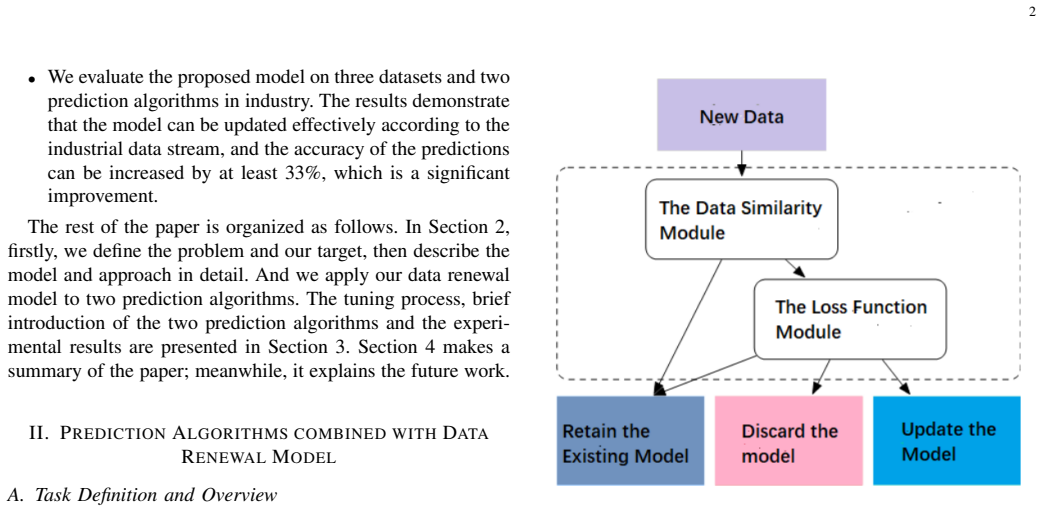
The central object is the data renewal model itself, implemented as two algorithms: Algorithm 1 decides the update flag from similarity and loss-change thresholds, and Algorithm 2 controls batch accumulation and model replacement. Its two signals are the similarity function — a modified Pearson correlation coefficient (absolute value) for numeric dimensions and an agreement-count ratio for binary dimensions, aggregated by weighted mean — and the loss function, with RMSE for continuous prediction and perceptual loss for classification. The loss-change rate $LC = |L_n - L_m|/L_m$, compared against thresholds $x$ and $y$, determines whether to retain, update, or discard and retrain the model. This mechanism carries the argument by turning the vague notion that 'the data have drifted' into a concrete, threshold-based trigger for model renewal.

What would settle it

Take a fresh industrial dataset (or a later, held-out period from the same plant), fix the thresholds without tuning, and compare the renewal model against a static model; if RMSE or AUC does not improve by the claimed margin, the reported gains are threshold artifacts rather than a general property of the renewal model.

Watch

Extended reading notes

Core claim

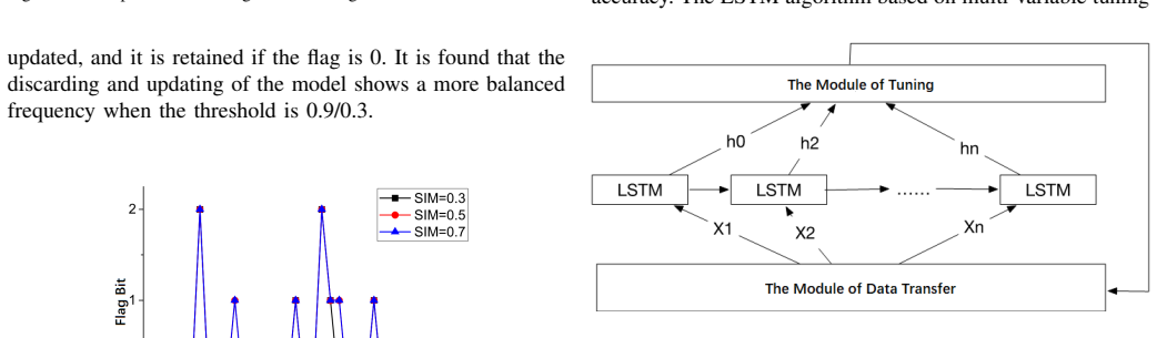
The central claim is that a prediction model's performance on industrial time-series data can be preserved and improved by a renewal model that combines two signals: the similarity between old and new data windows, measured by a modified Pearson correlation (for numeric data) or an agreement-count ratio (for binary data), and the relative change in the model's loss. When similarity falls below a threshold $z$, the algorithm computes the loss-change rate $LC = |L_n - L_m|/L_m$; if $LC$ exceeds an upper threshold $y$, the old model is discarded and retrained on the new data; if it lies between $x$ and $y$, the model is incrementally updated; otherwise it is kept. Applied to an LSTM-based yield predictor and a transfer-learning-based fault predictor, the paper reports that this mechanism reduces yield-prediction RMSE from 30.17 to 10.88 and raises fault-prediction AUC from 0.68 to 0.91, an improvement of at least 33%.

Load-bearing premise

The results rest on the assumption that the thresholds chosen by tuning on the boiler and generator datasets keep working on later windows of the same data, which is untested on new equipment.

Editorial extensions

If this is right

Industrial prediction systems using the renewal model should track equipment aging and abrasion automatically, reducing the need for manual recalibration.
Because the model only needs a similarity score and a loss value, it can be attached to any prediction algorithm that reports a loss, not just the two tested here.
The reported experiments indicate that update batch size matters: at 10,000, 50,000 and 100,000 pieces per batch, accuracy improves as data accumulate and then stabilizes.
Accuracy gains on both a regression task (yield, RMSE) and a classification task (faults, AUC) support the paper's claim of at least 33% improvement.

Reading between the lines

Editorial extensions of the paper, not claims the author makes directly.

The threshold values (similarity 0.5, loss rates 0.9/0.3) were tuned on the same boiler and generator datasets used for the evaluation, so the reported gains likely overstate performance on an unseen plant; a held-out validation would clarify.
The similarity signal, an absolute Pearson correlation, can stay high when a distribution shifts in mean or variance without changing linear correlation, so full-distribution drift measures could catch changes this model misses.
Because updates only trigger after a batch of data accumulates, the renewal model is a batch drift detector rather than a real-time one; fine-grained or streaming scenarios are not covered by the experiments.

Share X Bluesky LinkedIn Reddit HN

Signed reviews

No signed human review yet.

Editorial analysis

A structured set of objections, weighed in public.

Desk editor's note, referee report, and a circularity audit.

Desk Editor's Note

read the letter

Two things to know. First, the data renewal trigger is a reasonable, clearly specified combination of data-similarity and loss-change checks. Second, the experiments don't establish that the trigger helps: there is no static-model baseline, no periodic-retraining baseline, and the thresholds are tuned on the same datasets on which the gains are measured. The headline 'at least 33% improvement' is real as a raw before/after number, but it's not evidence for the renewal model specifically.

The paper does some things well. Algorithms 1 and 2 are explicit enough to reimplement. The similarity metric (absolute Pearson correlation for numeric, match ratio for binary) and the loss-change rate with three states (retain/update/discard) form a coherent decision rule. Applying it to two industrial predictors on real power-plant data is a sensible testbed, and the conclusion honestly notes that the thresholds are not self-adaptive.

The soft spots are load-bearing. The biggest issue is the missing control arms. Without a model that is never updated, or one retrained on a fixed schedule, or one simply retrained on the latest batch, the observed RMSE drop from 30.17 to 10.88 on the yield task and the AUC jump from 0.68 to 0.91 on the fault task could be caused by retraining alone, not by the renewal trigger. The secondary issue is in-sample threshold selection: Figures 3-6 tune the thresholds and then Tables II-III apply them to the same datasets, so the results partly measure fitted parameters. Also, the results are single runs with no error bars, and the '33.82%' on fault prediction is the only case that improves; two other rows show no change. The text has many typos and the base prediction algorithms are only roughly described, making replication harder than it should be.

Who might get value: someone working on practical model updating in industrial telemetry might take the decision rule as a starting point, but they should not regard the reported improvements as established. The paper would need a much stronger evaluation, with held-out thresholds, a periodic-retraining control, and repeated runs.

If I were the editor, I'd either desk reject on the inadequate evaluation or send back for major revision requiring new experiments. I would not spend referee time on the current version.

Referee Report

4 major / 5 minor

Summary. The paper proposes a "data renewal model" that decides when an existing prediction model should be updated or retrained on streaming industrial data. The decision is based on a similarity measure between old and new data windows and on the change rate of the loss function (Eq. 10). The model is presented as Algorithm 1 (update decision) and Algorithm 2 (lifelong update loop). It is applied to two base predictors: a multi-variable LSTM yield predictor and a transfer-learning-based fault predictor. Experiments on boiler and generator data report that the yield predictor's RMSE drops from 30.17 to 10.88 (Table II) and the fault predictor's AUC rises from 0.68 to 0.91 (Table III). The authors claim the accuracy can be increased by at least 33%.

Significance. If the central claim were established, a general retraining trigger for industrial prediction models would be practically useful, and the paper would complement existing work on concept drift and online learning. The paper does provide concrete algorithms, complexity analysis, and experiments on real industrial datasets. However, as submitted, the evidence does not support the causal attribution of the reported gains to the renewal trigger. The experiments lack the necessary control conditions, the thresholds are tuned on the same datasets used for evaluation, and the results are single runs without variability estimates. The headline improvement rests on one favorable row. These are load-bearing weaknesses for a paper whose contribution is the trigger mechanism rather than the base learners.

major comments (4)

[§III-C, §III-D, Tables II and III] The experiments contain no baseline in which the same base algorithms are (a) never updated, (b) retrained on a fixed schedule without the renewal trigger, or (c) retrained on the same newly accumulated data with the trigger disabled. The observed RMSE decrease from 30.17 to 10.88 and AUC increase from 0.68 to 0.91 are therefore equally consistent with the trivial explanation that retraining on newer or larger data improves accuracy. Because the paper's claimed contribution is the renewal trigger rather than the base predictor, this missing control is the central load-bearing weakness.
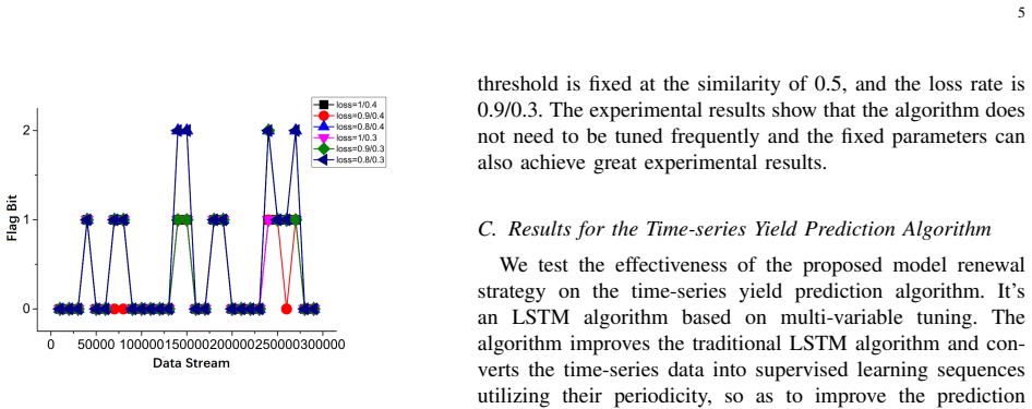
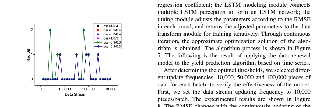
[§III-B, §III-C, §III-D] The similarity threshold z=0.5 and the loss-rate thresholds 0.9/0.3 are selected in Section III-B by observing update frequencies on the boiler and generator datasets, and the same datasets are then used in Sections III-C and III-D to evaluate the resulting model. This makes the reported RMSE and AUC improvements partly in-sample estimates of tuned parameters. A held-out validation split or a nested tuning procedure is needed to support the claim that fixed thresholds generalize.
[Tables II and III, Figures 8-12] All reported results are single runs without error bars, confidence intervals, or significance tests. Given that the base predictors are LSTM and transfer-learning networks with stochastic training, the improvements could reflect random variation. In particular, the abstract and introduction claim an accuracy increase of 'at least 33%', but this figure is supported only by Table III row No. 6 (AUC 0.68 to 0.91, a 33.82% relative increase); rows No. 4 and No. 5 show no improvement, so the claim is based on one favorable case.
[§III-C, §III-D] The evaluation protocol varies the data batch size (10,000, 50,000, 100,000 pieces per batch) but does not report the number of data points, model parameters, training epochs, or how the final RMSE/AUC values in Tables II and III were computed from the trajectories in Figures 8-12. Without this information the tables are not reproducible, and it is unclear whether the 'Accuracy' column reports the relative improvement over the initial row or something else.

minor comments (5)

[§II-B2, Eq. (10)] Equation (10) has a misplaced absolute value: it should read LC = |Ln - Lm| / Lm, not LC = |Ln - Lm / Lm|.
[§II-B1, Eq. (5)] Equation (5) has unbalanced parentheses in the numerator of the expectation, making the formula hard to parse; please correct the typography.
[§I] There are typos such as 'efﬁcieintly' and 'yeild' (Section IV), and the phrase 'the they are set' in Section II-B2 should read 'they are set'.
[§II-A, Eqs. (1)-(2)] The definition of the update condition in Eqs. (1)-(2) is informal: f(·) and f′(·) are introduced as if they denote learned functions, but the condition 'if f(·) = f′(·)' is not operational because the functions are never explicitly represented or compared.
[§III-A, Table I] Table I lists a 'Synthetic Industrial Generator Dataset' but the experimental sections describe only the boiler and generator datasets; please clarify whether the synthetic dataset is used anywhere and, if so, report its results.

Circularity Check

1 steps flagged · score 6.0 of 10

The thresholds tuned in Section III-B on the boiler and generator datasets are then used to report RMSE and AUC gains on the same datasets, making the claimed improvements in-sample rather than independent predictions.

fitted input called prediction [This occurs in Section III-B (threshold tuning) and Sections III-C and III-D (evaluation), including Tables II and III.]
"The thresholds will be adjusted according to the experiments. ... After tuning the prediction algorithm based on the data renewal model, the threshold is fixed at the similarity of 0.5, and the loss rate is 0.9/0.3. ... After determining the optimal thresholds, we selected different update frequencies, 10,000, 50,000 and 100,000 pieces of data for each batch, to verify the effectiveness of the model."

The update trigger parameters (similarity threshold z and loss-rate thresholds x, y) are explicitly tuned on the industrial boiler and generator datasets in Section III-B, with the paper stating 'The thresholds will be adjusted according to the experiments.' Sections III-C and III-D then report accuracy improvements on those same datasets, including an RMSE reduction from 30.17 to 10.88 (63.94%) and an AUC increase from 0.68 to 0.91 (33.82%), as evidence that the renewal model improves prediction accuracy. No held-out period, cross-validation split, or separate test set is introduced, so the reported 'updating accuracy' is an in-sample comparison after the trigger was calibrated to the evaluation data.

full rationale

The paper's model construction (Algorithm 1 with similarity threshold z and loss-rate thresholds x, y) is not definitionally identical to its output, and no self-citation chain or imported uniqueness theorem is load-bearing. The circularity lies in the evaluation protocol: Section III-B tunes the thresholds on the boiler and generator datasets, and Sections III-C and III-D report the RMSE and AUC improvements on exactly those datasets, with the paper stating 'The thresholds will be adjusted according to the experiments.' This fits the fitted-input-called-prediction pattern: the 'prediction' of improved accuracy is partly a consequence of calibrating the trigger parameters on the same data that are later used to measure the gain. The introduction promises a comparison 'between the learning models with and without a data renewal model,' but no such baseline arm appears in Sections III-C or III-D, so even a properly held-out threshold choice would not show that the renewal trigger, rather than plain retraining on recent data, causes the gains. The headline 'at least 33%' additionally rests on a single favorable row (Table III, No. 6) with no repeated runs or variability estimates. These issues make the central experimental claim partially circular, but the method itself does not reduce to its inputs by definition, so a moderate score of 6 is appropriate.

Assumptions & free parameters 4 free parameters · 4 assumptions · 0 invented entities

The model's behavior is controlled by three thresholds and a batch size, all chosen by the authors on the experimental data; no new physical or mathematical entities are introduced. The key assumptions are that similarity and loss-change statistics capture the need to update, and that retraining improves accuracy when thresholds are crossed.

free parameters (4)

Similarity threshold z = 0.5
Tuned on the boiler and generator datasets in Section III-B to balance update frequency; used in Algorithm 1 to decide whether to evaluate loss.
Loss change upper threshold y = 0.9
Tuned in Section III-B; if LC > y, the model is discarded and retrained.
Loss change lower threshold x = 0.3
Tuned in Section III-B; if x < LC < y, the model is updated with new data; if LC < x, the model is retained.
Minimum data batch size L = 10,000 / 50,000 / 100,000
Algorithm 2 waits until this many new samples arrive before checking similarity; the value is varied across experiments and affects results.

assumptions (4)

domain assumption Industrial time-series data are temporally correlated and model performance degrades as equipment conditions change over time.
Stated in the Introduction as motivation; the entire renewal model depends on this drift actually occurring in the datasets.
ad hoc to paper Absolute Pearson correlation (Equation 5) and the binary matching rate (Equation 3) adequately measure the distribution change relevant to model performance.
No justification or comparison to other drift measures; used as the trigger signal in Algorithm 1.
ad hoc to paper The loss change rate LC = |Ln - Lm| / Lm computed on new data predicts future model quality, and retraining when LC exceeds thresholds improves or maintains accuracy.
Core decision rule; no proof or robustness analysis; Ln is obtained by putting new data into the model, which is not precisely specified.
standard math Pearson correlation and standard loss definitions are valid statistical tools.
Background math, no issue.

how reviews work

0 comments

Cite this review

Pith. "Pith review of A General Data Renewal Model for Prediction Algorithms in Industrial Data Analytics." pith.science (2026). https://pith.science/paper/UHBK3Y4T

@misc{pith2026190808368,
  author       = {Pith},
  title        = {Pith review of: A General Data Renewal Model for Prediction Algorithms in Industrial Data Analytics},
  year         = {2026},
  howpublished = {\url{https://pith.science/paper/UHBK3Y4T}},
  note         = {Machine review of arXiv:1908.08368}
}

read the original abstract

In industrial data analytics, one of the fundamental problems is to utilize the temporal correlation of the industrial data to make timely predictions in the production process, such as fault prediction and yield prediction. However, the traditional prediction models are fixed while the conditions of the machines change over time, thus making the errors of predictions increase with the lapse of time. In this paper, we propose a general data renewal model to deal with it. Combined with the similarity function and the loss function, it estimates the time of updating the existing prediction model, then updates it according to the evaluation function iteratively and adaptively. We have applied the data renewal model to two prediction algorithms. The experiments demonstrate that the data renewal model can effectively identify the changes of data, update and optimize the prediction model so as to improve the accuracy of prediction.

Figures

Figures reproduced from arXiv: 1908.08368 by the authors.

**Figure 2.** The State-determining Schematic Diagram of the Loss Function [PITH_FULL_IMAGE:figures/full_fig_p003_2.png] view at source ↗

**Figure 3.** The Impact of the Similarity for Algorithm 1 [PITH_FULL_IMAGE:figures/full_fig_p004_3.png] view at source ↗

Figures from the paper (7 more)

**Figure 4.** Figure 4: The Impact of the Change Rate for Algorithm 1 [PITH_FULL_IMAGE:figures/full_fig_p005_4.png]

**Figure 7.** Figure 7: The Procedure of the Time-series Yield Prediction Algorithm [PITH_FULL_IMAGE:figures/full_fig_p005_7.png]

**Figure 6.** Figure 6: The Impact of the Change Rate for Algorithm 2 [PITH_FULL_IMAGE:figures/full_fig_p005_6.png]

**Figure 10.** Figure 10: The Schematic Diagram of the Transfer Learning Based Fault [PITH_FULL_IMAGE:figures/full_fig_p006_10.png]

**Figure 9.** Figure 9: The Result at a Frequency of 50000 pieces/batch [PITH_FULL_IMAGE:figures/full_fig_p006_9.png]

**Figure 11.** Figure 11: The Result at a Frequency of 10000 pieces/batch [PITH_FULL_IMAGE:figures/full_fig_p007_11.png]

**Figure 12.** Figure 12: The Result at a Frequency of 50000 pieces/batch [PITH_FULL_IMAGE:figures/full_fig_p007_12.png]

Discussion (0). Continue with ORCID to comment.

Reference graph

Works this paper leans on

30 extracted references · 27 canonical work pages

[1]

A review of machinery diagnostics and prognostics implemented on a centrifugal pump,

K. McKee, G. Forbes, I. Mazhar, R. Entwistle, and I. Howard, “A review of machinery diagnostics and prognostics implemented on a centrifugal pump,” in Engineering Asset Management 2011 . Springer, 2014, pp. 593–614

work page 2011
[2]

The analytic hierarchy process applied to maintenance strategy selection,

M. Bevilacqua and M. Braglia, “The analytic hierarchy process applied to maintenance strategy selection,” Reliability Engineering & System Safety, vol. 70, no. 1, pp. 71–83, 2000

work page 2000
[3]

Prognostics and health management of electronics,

M. Pecht, “Prognostics and health management of electronics,” Ency- clopedia of Structural Health Monitoring , 2009

work page 2009
[4]

Prognostic modelling options for remaining useful life estimation by industry,

J. Sikorska, M. Hodkiewicz, and L. Ma, “Prognostic modelling options for remaining useful life estimation by industry,” Mechanical Systems and Signal Processing , vol. 25, no. 5, pp. 1803–1836, 2011

work page 2011
[5]

Remaining useful life prediction for an adaptive skew-wiener process model,

Z. Huang, Z. Xu, X. Ke, W. Wang, and Y . Sun, “Remaining useful life prediction for an adaptive skew-wiener process model,” Mechanical Systems and Signal Processing , vol. 87, pp. 294–306, 2017

work page 2017
[6]

Residual life estimation based on a generalized wiener process with skew-normal random effects,

X. Wang, N. Balakrishnan, and B. Guo, “Residual life estimation based on a generalized wiener process with skew-normal random effects,” Communications in Statistics-Simulation and Computation , vol. 45, no. 6, pp. 2158–2181, 2016

work page 2016
[7]

Remain- ing useful life estimation based on a nonlinear diffusion degradation process,

X.-S. Si, W. Wang, C.-H. Hu, D.-H. Zhou, and M. G. Pecht, “Remain- ing useful life estimation based on a nonlinear diffusion degradation process,” IEEE Transactions on Reliability , vol. 61, no. 1, pp. 50–67, 2012

work page 2012
[8]

Fault detection for a class of uncertain nonlinear markovian jump stochastic systems with mode-dependent time delays and sensor saturation,

G. Zhuang, Y . Li, and Z. Li, “Fault detection for a class of uncertain nonlinear markovian jump stochastic systems with mode-dependent time delays and sensor saturation,” International Journal of Systems Science , vol. 47, no. 7, pp. 1514–1532, 2016

work page 2016

Show all 30 references

[9]

A manufacturing big data solution for active preventive maintenance,

J. Wan, S. Tang, D. Li, S. Wang, C. Liu, H. Abbas, and A. V . Vasilakos, “A manufacturing big data solution for active preventive maintenance,” IEEE Transactions on Industrial Informatics , vol. 13, no. 4, pp. 2039– 2047, 2017

2017
[10]

An automated auto-encoder correlation-based health-monitoring and prognostic method for machine bearings,

R. M. Hasani, G. Wang, and R. Grosu, “An automated auto-encoder correlation-based health-monitoring and prognostic method for machine bearings,” arXiv preprint arXiv:1703.06272 , 2017

2017 arXiv
[11]

Opportunistic maintenance for wind turbines considering imperfect, reliability-based maintenance,

C. Zhang, W. Gao, S. Guo, Y . Li, and T. Yang, “Opportunistic maintenance for wind turbines considering imperfect, reliability-based maintenance,” Renewable energy, vol. 103, pp. 606–612, 2017

2017
[12]

Prognostic health management of aircraft power generators,

T. D. Batzel and D. C. Swanson, “Prognostic health management of aircraft power generators,” IEEE Transactions on Aerospace and Electronic Systems, vol. 45, no. 2, 2009

2009
[13]

Reliability of manu- facturing equipment in complex environments,

J. P. Kharoufeh, S. M. Cox, and M. E. Oxley, “Reliability of manu- facturing equipment in complex environments,” Annals of Operations Research, vol. 209, no. 1, pp. 231–254, 2013

2013
[14]

Learning transferable features with deep adaptation networks,

M. Long, C. Yue, J. Wang, and M. I. Jordan, “Learning transferable features with deep adaptation networks,” 2015

2015
[15]

Transfer learning with neural networks for bearing fault diagnosis in changing working conditions,

Z. Ran, H. Tao, L. Wu, and G. Yong, “Transfer learning with neural networks for bearing fault diagnosis in changing working conditions,” IEEE Access, vol. PP, no. 99, pp. 1–1, 2017

2017
[16]

Lifelong machine learning,

Z. Chen and B. Liu, “Lifelong machine learning,” Synthesis Lectures on Artiﬁcial Intelligence and Machine Learning , vol. 10, no. 3, pp. 1–145, 2016

2016
[17]

Lifelong machine learning: a paradigm for continuous learning,

B. Liu, “Lifelong machine learning: a paradigm for continuous learning,” Frontiers of Computer Science , vol. 11, no. 3, pp. 359–361, 2017

2017
[18]

Lifelong machine learning systems: Beyond learning algorithms

D. L. Silver, Q. Yang, and L. Li, “Lifelong machine learning systems: Beyond learning algorithms.” in AAAI Spring Symposium: Lifelong Machine Learning, vol. 13, 2013, p. 05

2013
[19]

Efﬁcient representations for lifelong learning and autoencoding,

M.-F. Balcan, A. Blum, and S. Vempala, “Efﬁcient representations for lifelong learning and autoencoding,” in Conference on Learning Theory, 2015, pp. 191–210

2015
[20]

Lifelong machine learning with adaptive multi-agent systems,

N. R. Verstaevel, J. Boes, J. Nigon, D. d’Amico, and M.-P. Gleizes, “Lifelong machine learning with adaptive multi-agent systems,” 2017

2017
[21]

The parallel transfer of task knowledge using dynamic learning rates based on a measure of relatedness,

D. L. Silver and R. E. Mercer, “The parallel transfer of task knowledge using dynamic learning rates based on a measure of relatedness,” in Learning to learn . Springer, 1996, pp. 213–233

1996
[22]

Transfer of learning by composing solutions of elemental sequential tasks,

S. P. Singh, “Transfer of learning by composing solutions of elemental sequential tasks,” Machine Learning, vol. 8, no. 3-4, pp. 323–339, 1992

1992
[23]

The task rehearsal method of life- long learning: Overcoming impoverished data,

D. L. Silver and R. E. Mercer, “The task rehearsal method of life- long learning: Overcoming impoverished data,” in Conference of the Canadian Society for Computational Studies of Intelligence . Springer, 2002, pp. 90–101

2002
[24]

A fault prediction method based on modiﬁed genetic algorithm using bp neural network algorithm,

Q. Liu, Z. Feng, L. Min, and W. Shen, “A fault prediction method based on modiﬁed genetic algorithm using bp neural network algorithm,” in IEEE International Conference on Systems , 2017. 8

2017
[25]

Deep convolutional neural networks for computer-aided detection: Cnn architectures, dataset characteristics and transfer learning,

H. C. Shin, H. R. Roth, M. Gao, L. Lu, Z. Xu, I. Nogues, J. Yao, D. Mollura, and R. M. Summers, “Deep convolutional neural networks for computer-aided detection: Cnn architectures, dataset characteristics and transfer learning,” IEEE Transactions on Medical Imaging , vol. 35, ...

2016
[26]

Long short-term memory neural network for trafﬁc speed prediction using remote microwave sensor data,

X. Ma, Z. Tao, Y . Wang, H. Yu, and Y . Wang, “Long short-term memory neural network for trafﬁc speed prediction using remote microwave sensor data,” Transportation Research Part C , vol. 54, pp. 187–197, 2015

2015
[27]

Are loss functions all the same?

L. Rosasco, E. D. Vito, A. Caponnetto, M. Piana, and A. Verri, “Are loss functions all the same?” Neural Computation , vol. 16, no. 5, pp. 1063–1076, 2004

2004
[28]

Loss functions for binary classiﬁcation and class probability estimation,

Y . Shen, “Loss functions for binary classiﬁcation and class probability estimation,” Ph.D. dissertation, University of Pennsylvania, 2005

2005
[29]

On the design of loss functions for classiﬁcation: theory, robustness to outliers, and savageboost,

H. Masnadi-Shirazi and N. Vasconcelos, “On the design of loss functions for classiﬁcation: theory, robustness to outliers, and savageboost,” in Advances in neural information processing systems , 2009, pp. 1049– 1056

2009
[30]

An introduction to roc analysis,

T. Fawcett, “An introduction to roc analysis,” Pattern recognition letters, vol. 27, no. 8, pp. 861–874, 2006

2006

Pith tools

Reviewed August 14, 2026 · model on record in the stance chip above.

[1] [1]

A review of machinery diagnostics and prognostics implemented on a centrifugal pump,

K. McKee, G. Forbes, I. Mazhar, R. Entwistle, and I. Howard, “A review of machinery diagnostics and prognostics implemented on a centrifugal pump,” in Engineering Asset Management 2011 . Springer, 2014, pp. 593–614

work page 2011

[2] [2]

The analytic hierarchy process applied to maintenance strategy selection,

M. Bevilacqua and M. Braglia, “The analytic hierarchy process applied to maintenance strategy selection,” Reliability Engineering & System Safety, vol. 70, no. 1, pp. 71–83, 2000

work page 2000

[3] [3]

Prognostics and health management of electronics,

M. Pecht, “Prognostics and health management of electronics,” Ency- clopedia of Structural Health Monitoring , 2009

work page 2009

[4] [4]

Prognostic modelling options for remaining useful life estimation by industry,

J. Sikorska, M. Hodkiewicz, and L. Ma, “Prognostic modelling options for remaining useful life estimation by industry,” Mechanical Systems and Signal Processing , vol. 25, no. 5, pp. 1803–1836, 2011

work page 2011

[5] [5]

Remaining useful life prediction for an adaptive skew-wiener process model,

Z. Huang, Z. Xu, X. Ke, W. Wang, and Y . Sun, “Remaining useful life prediction for an adaptive skew-wiener process model,” Mechanical Systems and Signal Processing , vol. 87, pp. 294–306, 2017

work page 2017

[6] [6]

Residual life estimation based on a generalized wiener process with skew-normal random effects,

X. Wang, N. Balakrishnan, and B. Guo, “Residual life estimation based on a generalized wiener process with skew-normal random effects,” Communications in Statistics-Simulation and Computation , vol. 45, no. 6, pp. 2158–2181, 2016

work page 2016

[7] [7]

Remain- ing useful life estimation based on a nonlinear diffusion degradation process,

X.-S. Si, W. Wang, C.-H. Hu, D.-H. Zhou, and M. G. Pecht, “Remain- ing useful life estimation based on a nonlinear diffusion degradation process,” IEEE Transactions on Reliability , vol. 61, no. 1, pp. 50–67, 2012

work page 2012

[8] [8]

Fault detection for a class of uncertain nonlinear markovian jump stochastic systems with mode-dependent time delays and sensor saturation,

G. Zhuang, Y . Li, and Z. Li, “Fault detection for a class of uncertain nonlinear markovian jump stochastic systems with mode-dependent time delays and sensor saturation,” International Journal of Systems Science , vol. 47, no. 7, pp. 1514–1532, 2016

work page 2016