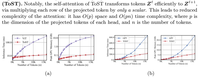
Principles and Practice of Deep Representation Learning: or a Mathematical Theory of Memory
Pith reviewed 2026-06-28 03:04 UTC · model grok-4.3
The pith
Deep neural network architectures follow from optimization and information theory, reducing design to linear algebra and calculus.
A machine-rendered reading of the paper's core claim, the machinery that carries it, and where it could break.
Core claim
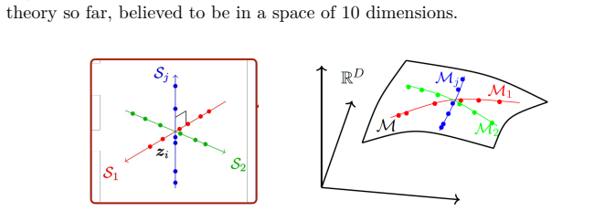
The mechanisms of large deep networks are understood through representation learning, arguably the single most important factor in their empirical power, and the design principles of modern neural network architectures are explained through optimization and information theory, turning the process of architecture development into undergraduate-level linear algebra and calculus exercises once the principles are introduced.
What carries the argument
Representation learning mechanisms derived from optimization and information theory, which carries the argument by supplying the core internal operations that explain why deep networks work.
If this is right
- Architecture development reduces to standard undergraduate linear algebra and calculus exercises.
- New methods and models become efficient, interpretable, and controllable by design while matching or exceeding black-box performance.
- Problems in various domains can be solved using these derived principles in more systematic ways.
Where Pith is reading between the lines
- The same principles might be extended to derive architectures for generative models without separate empirical search.
- If the derivations hold, they could provide a route to provable guarantees on model behavior that current empirical approaches lack.
- Connections to memory mechanisms in the title suggest potential links to classical theories of storage and retrieval in linear systems.
Load-bearing premise
The empirical power of deep learning is driven primarily by representation learning mechanisms that can be fully derived from optimization and information theory without requiring additional empirical tuning or domain-specific assumptions.
What would settle it
A high-performing deep network architecture that cannot be derived or explained using only optimization and information theory, or whose performance requires extra assumptions outside those frameworks, would falsify the central claim.
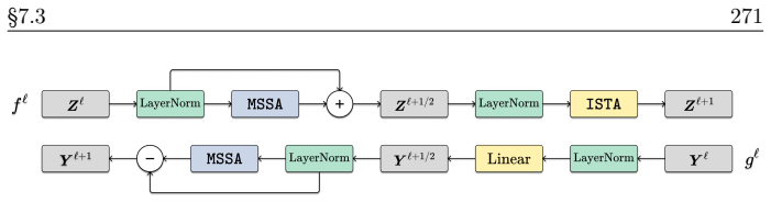
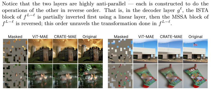
Figures


read the original abstract
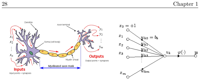
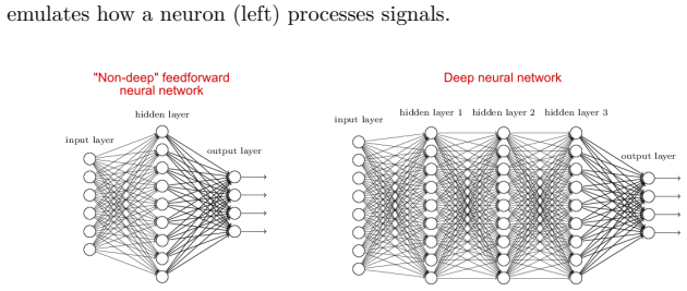
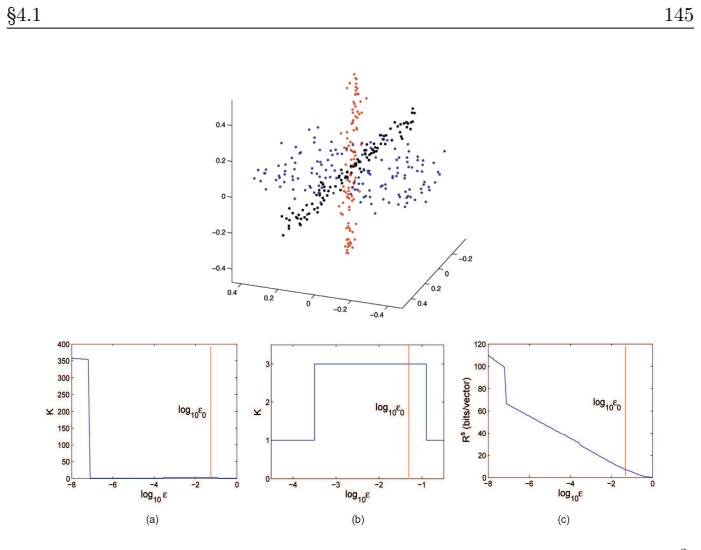
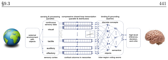
In the current era of deep learning and especially generative models, there is significant investment in training very large deep neural networks. Thus far, such models have been "black boxes" that are difficult to understand in the sense that they have opaque internal mechanisms, leading to difficulties in interpretability, reliability, and control. Naturally, this lack of understanding has led to both hype and fear. This book is an attempt to "open the black box" and understand the mechanisms of large deep networks, through the perspective of representation learning, which is a major factor - arguably the single most important one - in the empirical power of deep learning models. A brief outline of this book is as follows. Chapter 1 will summarize the threads that underlie the whole text. Chapters 2, 3, 4, 5, and 6 will explain the design principles of modern neural network architectures through optimization and information theory, reducing the process of architecture development (long having been described as a sort of "alchemy") to undergraduate-level linear algebra and calculus exercises once the underlying principles are introduced. Chapters 7 and 8 will discuss applications of these principles to solve problems in more paradigmatic ways, obtaining new methods and models which are efficient, interpretable, and controllable by design, and yet no less - sometimes even more - powerful than the black-box models they resemble. Chapter 9 will discuss potential future directions for deep learning, the role of representation learning, as well as some open problems.
Editorial analysis
A structured set of objections, weighed in public.
Referee Report
Summary. The manuscript is a book-length work proposing a mathematical theory of representation learning and memory in deep neural networks. Chapter 1 summarizes underlying threads; chapters 2–6 claim to derive the design principles of modern architectures from optimization and information theory, reducing architecture development to undergraduate linear algebra and calculus exercises; chapters 7–8 apply these principles to obtain new efficient, interpretable models; chapter 9 discusses future directions and open problems.
Significance. If the promised derivations in chapters 2–6 were supplied and shown to be parameter-free reductions grounded only in optimization and information theory, the work would offer a valuable contribution by replacing ad-hoc architecture search with explicit mathematical principles, improving interpretability and control. The framing around representation learning as the core driver of empirical success is a coherent organizing lens. No machine-checked proofs, reproducible code, or falsifiable predictions are present in the supplied text.
major comments (1)
- [Abstract] Abstract and chapter outline: the central claim that chapters 2–6 reduce architecture design to undergraduate linear algebra and calculus via optimization and information theory is asserted without any equations, derivations, worked examples, or even high-level proof sketches. This absence makes the load-bearing promise of the manuscript unverifiable from the text.
Simulated Author's Rebuttal
We thank the referee for their review and for identifying the central verifiability issue in the supplied text. We address the major comment below.
read point-by-point responses
-
Referee: [Abstract] Abstract and chapter outline: the central claim that chapters 2–6 reduce architecture design to undergraduate linear algebra and calculus via optimization and information theory is asserted without any equations, derivations, worked examples, or even high-level proof sketches. This absence makes the load-bearing promise of the manuscript unverifiable from the text.
Authors: The supplied manuscript text consists of the abstract and chapter outline; the detailed derivations promised for chapters 2–6 are not present. We agree that this renders the central claim unverifiable from the current text. We will revise by expanding the outline in Chapter 1 to incorporate high-level proof sketches and at least two worked examples (one from optimization and one from information theory) that illustrate the claimed reduction to undergraduate linear algebra and calculus. These additions will be placed before the chapter summaries so that readers can assess the approach without needing the full later chapters. revision: yes
Circularity Check
No significant circularity detected
full rationale
The abstract and chapter outline describe a high-level program for deriving neural architecture principles from optimization and information theory, but supply no equations, fitted parameters, self-citations, or uniqueness theorems that could be inspected for reduction to inputs. No load-bearing derivation chain is exhibited in the provided text, so the claimed reduction to undergraduate linear algebra remains an unverified assertion rather than a demonstrated circularity. This is the expected honest non-finding when concrete steps are absent.
Axiom & Free-Parameter Ledger
Reference graph
Works this paper leans on
-
[1]
Direct linear transformation from comparator coordinates into object space coordinates in close-range photogrammetry
[AKH15] Yousset I Abdel-Aziz, Hauck Michael Karara, and Michael Hauck. “Direct linear transformation from comparator coordinates into object space coordinates in close-range photogrammetry” . Pho- togrammetric engineering & remote sensing 81.2 (2015), pp. 103–
2015
-
[2]
Learning Sparsely Used Overcomplete Dictio- naries via Alternating Minimization
[AAJ+16] Alekh Agarwal, Animashree Anandkumar, Prateek Jain, and Pra- neeth Netrapalli. “Learning Sparsely Used Overcomplete Dictio- naries via Alternating Minimization” . SIAM Journal on Opti- mization 26.4 (2016), pp. 2775–2799. eprint: https://doi.org/ 10.1137/140979861. [AEB06] Michal Aharon, Michael Elad, and Alfred Bruckstein. “K-SVD: An algorithm f...
-
[3]
Why do deep convolutional networks generalize so poorly to small image transformations?
Proceedings of Machine Learning Research. Paris, France: PMLR, July 2015, pp. 113–149. [A W18] Aharon Azulay and Yair Weiss. “Why do deep convolutional networks generalize so poorly to small image transformations?” arXiv preprint arXiv:1805.12177 (2018). [BJC85] B. Ans, J. Hérault, and C. Jutten. “Architectures neuromimé- tiques adaptatives : Détection de...
arXiv 2015
-
[4]
A fast iterative shrinkage-thresholding algorithm for linear inverse problems
[BT09] Amir Beck and Marc Teboulle. “A fast iterative shrinkage-thresholding algorithm for linear inverse problems” . SIAM journal on imaging sciences 2.1 (2009), pp. 183–202. [BHM+19] Mikhail Belkin, Daniel Hsu, Siyuan Ma, and Soumik Mandal. “Reconciling modern machine-learning practice and the classical bias–variance trade-off” .Proceedings of the Natio...
2009
-
[5]
Computation of channel capacity and rate-distortion functions
arXiv: 2409.20325 [cs.LG] . [Bla72] R. Blahut. “Computation of channel capacity and rate-distortion functions” .IEEE Transactions on Information Theory 18.4 (1972), pp. 460–473. [BRL+23] Andreas Blattmann, Robin Rombach, Huan Ling, Tim Dockhorn, Seung Wook Kim, Sanja Fidler, and Karsten Kreis. “Align your latents: High-resolution video synthesis with late...
Pith/arXiv arXiv 1972
-
[6]
Classifier-Free Guid- ance is a Predictor-Corrector
[BN24b] Arwen Bradley and Preetum Nakkiran. “Classifier-Free Guid- ance is a Predictor-Corrector” . arXiv [cs.LG] (Aug. 2024). arXiv: 2408.09000 [cs.LG] . [BN20] Guy Bresler and Dheeraj Nagaraj. “Sharp representation theo- rems for relu networks with precise dependence on depth” . Pro- ceedings of the 34th International Conference on Neural Infor- mation ...
arXiv 2024
-
[7]
2020, pp
Red Hook, NY, USA: Curran Associates Inc., Dec. 2020, pp. 10697–10706. [BB11] Haim Brezis and Haim Brézis. Functional analysis, Sobolev spaces and partial differential equations . Vol
2020
-
[8]
Matrix Calculus (for Machine Learning and Beyond)
[BEJ25] Paige Bright, Alan Edelman, and Steven G Johnson. “Matrix Calculus (for Machine Learning and Beyond)” . arXiv preprint arXiv:2501.14787 (2025). [BDS19] Andrew Brock, Jeff Donahue, and Karen Simonyan. “Large Scale GAN Training for High Fidelity Natural Image Synthesis” . Inter- national Conference on Learning Representations (ICLR)
arXiv 2025
-
[9]
Lan- guage models are few-shot learners
[BMR+20] Tom B. Brown, Benjamin Mann, Nick Ryder, Melanie Subbiah, Jared Kaplan, Prafulla Dhariwal, Arvind Neelakantan, Pranav Shyam, Girish Sastry, Amanda Askell, Sandhini Agarwal, Ariel Herbert-Voss, Gretchen Krueger, Tom Henighan, Rewon Child, Aditya Ramesh, Daniel M. Ziegler, Jeffrey Wu, Clemens Winter, Christopher Hesse, Mark Chen, Eric Sigler, Mateu...
Pith/arXiv arXiv 2005
-
[10]
Invariant Scattering Convo- lution Networks
[BM13] Joan Bruna and Stéphane Mallat. “Invariant Scattering Convo- lution Networks” . IEEE Transactions on Pattern Analysis and Machine Intelligence 35.8 (2013), pp. 1872–1886. §B.3 515 [BGW21] Sam Buchanan, Dar Gilboa, and John Wright. “Deep Networks and the Multiple Manifold Problem” . International Conference on Learning Representations
2013
-
[11]
On the edge of memorization in diffusion models
[BPM+25] Sam Buchanan, Druv Pai, Yi Ma, and Valentin De Bortoli. “On the edge of memorization in diffusion models” . arXiv preprint arXiv:2508.17689 (2025). [CD91] M. Frank Callier and A. Charles Desoer. Linear System Theory . Springer-Verlag,
arXiv 2025
-
[12]
Decoding by linear programming
[CT05a] E. Candès and T. Tao. “Decoding by linear programming” . IEEE Transactions on Information Theory 51.12 (2005). [CT05b] E. Candès and T. Tao. “Error Correction via Linear Program- ming” .IEEE Symposium on FOCS (2005), pp. 295–308. [CMM+21] Mathilde Caron, Ishan Misra, Julien Mairal, Priya Goyal, Piotr Bojanowski, and Armand Joulin. Unsupervised Lea...
2005
-
[13]
Emerging prop- erties in self-supervised vision transformers
09882 [cs.CV] . [CTM+21] Mathilde Caron, Hugo Touvron, Ishan Misra, Hervé Jégou, Julien Mairal, Piotr Bojanowski, and Armand Joulin. “Emerging prop- erties in self-supervised vision transformers” . Proceedings of the IEEE/CVF international conference on computer vision . 2021, pp. 9650–9660. [Cha66] Gregory J. Chaitin. “On the Length of Programs for Compu...
Pith/arXiv arXiv 2021
-
[14]
Score approximation, estimation and distribution recovery of diffusion models on low-dimensional data
[CHZ+23] Minshuo Chen, Kaixuan Huang, Tuo Zhao, and Mengdi Wang. “Score approximation, estimation and distribution recovery of diffusion models on low-dimensional data” . International Con- ference on Machine Learning . PMLR. 2023, pp. 4672–4712. [CRB+18] Ricky TQ Chen, Yulia Rubanova, Jesse Bettencourt, and David K Duvenaud. “Neural ordinary differential...
2023
-
[15]
Exploring low-dimensional subspace in diffusion mod- els for controllable image editing
[CZG+24] Siyi Chen, Huijie Zhang, Minzhe Guo, Yifu Lu, Peng Wang, and Qing Qu. “Exploring low-dimensional subspace in diffusion mod- els for controllable image editing” . Advances in Neural Informa- tion Processing Systems 37 (2024), pp. 27340–27371. [CZL+25] Siyi Chen, Yimeng Zhang, Sijia Liu, and Qing Qu. “The Dual Power of Interpretable Token Embedding...
arXiv 2024
-
[16]
Group equivariant convolutional networks
[CW16a] Taco Cohen and Max Welling. “Group equivariant convolutional networks” .International Conference on Machine Learning . 2016, pp. 2990–2999. [CW16b] Taco Cohen and Max Welling. “Group equivariant convolutional networks” .International conference on machine learning . PMLR. 2016, pp. 2990–2999. [CW16c] Taco S. Cohen and Max Welling. “Group Equivaria...
Pith/arXiv arXiv 2016
-
[17]
Support-Vector Networks
07576. [CV95] Corinna Cortes and Vladimir Vapnik. “Support-Vector Networks” . Mach. Learn. 20.3 (1995), pp. 273–297. [CT91] T. Cover and J. Thomas. Elements of Information Theory . Wiley Series in Telecommunications,
1995
-
[18]
Geometrical and Statistical Properties of Sys- tems of Linear Inequalities with Applications in Pattern Recog- nition
[Cov64] Thomas Cover. “Geometrical and Statistical Properties of Sys- tems of Linear Inequalities with Applications in Pattern Recog- nition” .IEEE TRANSACTIONS ON ELECTRONIC COMPUT- ERS (1964). [Cyb89] George V. Cybenko. “Approximation by superpositions of a sig- moidal function” .Mathematics of Control, Signals and Systems 2 (1989), pp. 303–314. [D D00]...
1964
-
[19]
Distributional Diffusion Models with Scoring Rules
Curran Associates, Inc., 2023, pp. 288–313. [DGG+25] Valentin De Bortoli, Alexandre Galashov, J Swaroop Guntupalli, Guangyao Zhou, Kevin Murphy, Arthur Gretton, and Arnaud Doucet. “Distributional Diffusion Models with Scoring Rules” . arXiv preprint arXiv:2502.02483 (2025). [DCM+23] Aaron Defazio, Ashok Cutkosky, Harsh Mehta, and Konstantin Mishchenko. “O...
arXiv 2023
-
[20]
Gromov– Wasserstein distances between Gaussian distributions
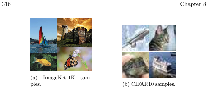
[DDS22] Julie Delon, Agnes Desolneux, and Antoine Salmona. “Gromov– Wasserstein distances between Gaussian distributions” . Journal of Applied Probability 59.4 (2022), pp. 1178–1198. [DDS+09a] J. Deng, W. Dong, R. Socher, L.-J. Li, K. Li, and L. Fei-Fei. “Im- ageNet: A Large-Scale Hierarchical Image Database” . CVPR09
2022
-
[21]
ImageNet: A Large-Scale Hierarchical Image Database
[DDS+09b] Jia Deng, Wei Dong, Richard Socher, Li-Jia Li, Kai Li, and Li Fei-Fei. “ImageNet: A Large-Scale Hierarchical Image Database” . Proceedings of the IEEE/CVF Conference on Computer Vision and Pattern Recognition (CVPR) . 2009, pp. 248–255. [DCL+19] Jacob Devlin, Ming-Wei Chang, Kenton Lee, and Kristina Toutanova. “Bert: Pre-training of deep bidirec...
2009
-
[22]
Sparse components of images and optimal atomic decompositions
[Don01] D L Donoho. “Sparse components of images and optimal atomic decompositions” . Constructive approximation 17.3 (Jan. 2001), pp. 353–382. [DVD+98] D L Donoho, M Vetterli, R A DeVore, and I Daubechies. “Data compression and harmonic analysis” . IEEE transactions on in- formation theory / Professional Technical Group on Information Theory 44.6 (Oct. 1...
2001
-
[23]
Google scanned objects: A high-quality dataset of 3d scanned household items
[DFK+22] Laura Downs, Anthony Francis, Nate Koenig, Brandon Kinman, Ryan Hickman, Krista Reymann, Thomas B McHugh, and Vin- cent Vanhoucke. “Google scanned objects: A high-quality dataset of 3d scanned household items” . 2022 International Conference on Robotics and Automation (ICRA). IEEE. 2022, pp. 2553–2560. [DSC22] Shiv Ram Dubey, Satish Kumar Singh, ...
Pith/arXiv arXiv 2022
-
[24]
[EHO+22a] Nelson Elhage, Tristan Hume, Catherine Olsson, Nicholas Schiefer, Tom Henighan, Shauna Kravec, Zac Hatfield-Dodds, Robert Lasenby, Dawn Drain, Carol Chen, et al. “Toy models of superposition” . arXiv preprint arXiv:2209.10652 (2022). [EHO+22b] Nelson Elhage, Tristan Hume, Catherine Olsson, Nicholas Schiefer, Tom Henighan, Shauna Kravec, Zac Hatf...
Pith/arXiv arXiv 2022
-
[25]
Taming trans- formers for high-resolution image synthesis
[ERO21] Patrick Esser, Robin Rombach, and Bjorn Ommer. “Taming trans- formers for high-resolution image synthesis” . Proceedings of the IEEE/CVF conference on computer vision and pattern recogni- tion. 2021, pp. 12873–12883. [EGW+10] Mark Everingham, Luc Van Gool, Christopher K. I. Williams, John Winn, and Andrew Zisserman. The PASCAL Visual Object Classe...
2021
-
[26]
Diffusion models and the man- ifold hypothesis: Log-domain smoothing is geometry adaptive
arXiv: 0909.5206 [cs.CV] . [FPH+25] Tyler Farghly, Peter Potaptchik, Samuel Howard, George Deli- giannidis, and Jakiw Pidstrigach. “Diffusion models and the man- ifold hypothesis: Log-domain smoothing is geometry adaptive” . arXiv preprint arXiv:2510.02305 (2025). [FZS22] William Fedus, Barret Zoph, and Noam Shazeer. “Switch trans- formers: scaling to tri...
Pith/arXiv arXiv 2025
-
[27]
§B.3 521 [FCR20] Tanner Fiez, Benjamin Chasnov, and Lillian Ratliff. “Implicit learning dynamics in stackelberg games: Equilibria characteriza- tion, convergence analysis, and empirical study” . International Conference on Machine Learning . PMLR. 2020, pp. 3133–3144. [FCR19] Tanner Fiez, Benjamin Chasnov, and Lillian J Ratliff. “Conver- gence of learning...
arXiv 2020
-
[28]
Scaling and evaluating sparse autoencoders
arXiv: 2304.14108 [cs.CV] . [GTT+25] Leo Gao, Tom Dupre la Tour, Henk Tillman, Gabriel Goh, Rajan Troll, Alec Radford, Ilya Sutskever, Jan Leike, and Jeffrey Wu. “Scaling and evaluating sparse autoencoders” . The Thirteenth In- ternational Conference on Learning Representations
-
[29]
Handbook of conver- gence theorems for (stochastic) gradient methods
[GG23] Guillaume Garrigos and Robert M Gower. “Handbook of conver- gence theorems for (stochastic) gradient methods” . arXiv preprint arXiv:2301.11235 (2023). [GWX+25] Zheng Geng, Nan Wang, Shaocong Xu, Chongjie Ye, Bohan Li, Zhaoxi Chen, Sida Peng, and Hao Zhao. “One View, Many Worlds: Single-Image to 3D Object Meets Generative Domain Random- ization for...
-
[30]
[GPM+14b] Ian Goodfellow, Jean Pouget-Abadie, Mehdi Mirza, Bing Xu, David Warde-Farley, Sherjil Ozair, Aaron Courville, and Yoshua Bengio. “Generative adversarial nets” . Advances in neural infor- mation processing systems . 2014, pp. 2672–2680. [GDG+17] Priya Goyal, Piotr Dollár, Ross Girshick, Pieter Noordhuis, Lukasz Wesolowski, Aapo Kyrola, Andrew Tul...
Pith/arXiv arXiv 2014
-
[31]
Should Penalized Least Squares Regression be Interpreted as Maximum A Posteriori Estimation?
[Gri11] Rémi Gribonval. “Should Penalized Least Squares Regression be Interpreted as Maximum A Posteriori Estimation?” IEEE trans- actions on signal processing: a publication of the IEEE Signal Processing Society 59.5 (May 2011), pp. 2405–2410. §B.3 523 [GJB15] Remi Gribonval, Rodolphe Jenatton, and Francis Bach. “Sparse and spurious: Dictionary learning ...
2011
-
[32]
Competitive Learning: From Interactive Ac- tivation to Adaptive Resonance
[Gro87] Stephen Grossberg. “Competitive Learning: From Interactive Ac- tivation to Adaptive Resonance” . Cogn. Sci. 11 (1987), pp. 23–
1987
-
[33]
On memorization in diffusion models
[GDP+23] Xiangming Gu, Chao Du, Tianyu Pang, Chongxuan Li, Min Lin, and Ye Wang. “On memorization in diffusion models” . arXiv preprint arXiv:2310.02664 (2023). [GYR+23] Yuwei Guo, Ceyuan Yang, Anyi Rao, Zhengyang Liang, Yaohui Wang, Yu Qiao, Maneesh Agrawala, Dahua Lin, and Bo Dai. “Animatediff: Animate your personalized text-to-image diffusion models wi...
arXiv 2023
-
[34]
Masked autoencoders are scalable vision learners
[HCX+22] Kaiming He, Xinlei Chen, Saining Xie, Yanghao Li, Piotr Dol- lár, and Ross Girshick. “Masked autoencoders are scalable vision learners” .Proceedings of the IEEE/CVF conference on computer vision and pattern recognition . 2022, pp. 16000–16009. [HFW+19] Kaiming He, Haoqi Fan, Yuxin Wu, Saining Xie, and Ross Gir- shick. “Momentum contrast for unsup...
arXiv 2022
-
[35]
Gans trained by a two time- scale update rule converge to a local nash equilibrium
[HRU+17b] Martin Heusel, Hubert Ramsauer, Thomas Unterthiner, Bern- hard Nessler, and Sepp Hochreiter. “Gans trained by a two time- scale update rule converge to a local nash equilibrium” . Advances in neural information processing systems 30 (2017). [HS06] G. E. Hinton and R. R. Salakhutdinov. “Reducing the Dimen- sionality of Data with Neural Networks” ...
2017
-
[36]
Classifier-Free Diffusion Guid- ance
2020, pp. 6840–6851. [HS21] Jonathan Ho and Tim Salimans. “Classifier-Free Diffusion Guid- ance” .NeurIPS 2021 Workshop on Deep Generative Models and Downstream Applications
2020
-
[37]
Classifier-Free Diffusion Guid- ance
[HS22a] Jonathan Ho and Tim Salimans. “Classifier-Free Diffusion Guid- ance” .arXiv [cs.LG] (July 2022). arXiv: 2207.12598 [cs.LG] . [HS22b] Jonathan Ho and Tim Salimans. “Classifier-Free Diffusion Guid- ance” .NeurIPS 2021 Workshop on Deep Generative Models and Downstream Applications
Pith/arXiv arXiv 2022
-
[38]
Long Short-term Mem- ory
[HS97] Sepp Hochreiter and Jürgen Schmidhuber. “Long Short-term Mem- ory” .Neural computation 9 (Dec. 1997), pp. 1735–80. [HSD20] David Hong, Yue Sheng, and Edgar Dobriban. Selecting the num- ber of components in PCA via random signflips
1997
-
[39]
Lrm: Large reconstruction model for single image to 3d
arXiv: 2012.02985 [math.ST] . §B.3 525 [HZG+23] Yicong Hong, Kai Zhang, Jiuxiang Gu, Sai Bi, Yang Zhou, Difan Liu, Feng Liu, Kalyan Sunkavalli, Trung Bui, and Hao Tan. “Lrm: Large reconstruction model for single image to 3d” . arXiv preprint arXiv:2311.04400 (2023). [Hot33] H. Hotelling. “Analysis of a Complex of Statistical Variables into Principal Compo...
Pith/arXiv arXiv 2012
-
[40]
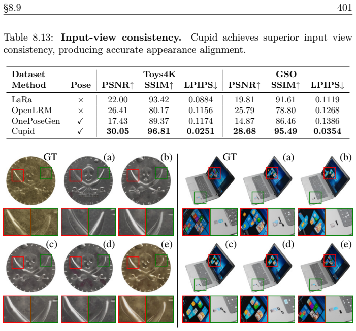
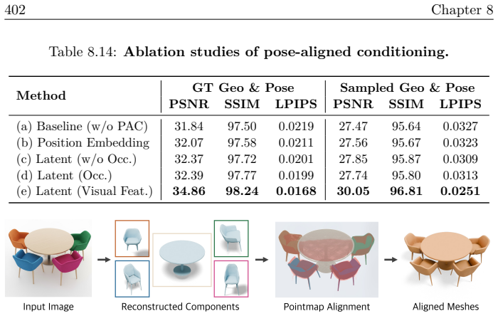
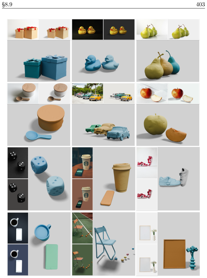
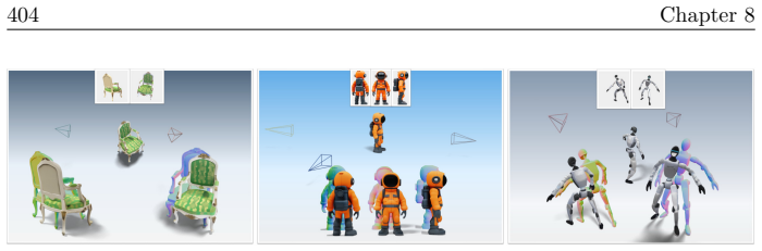
CUPID: Generative 3D Reconstruction via Joint Object and Pose Modeling
[HDZ+25] Binbin Huang, Haobin Duan, Yiqun Zhao, Zibo Zhao, Yi Ma, and Shenghua Gao. “CUPID: Generative 3D Reconstruction via Joint Object and Pose Modeling” .arXiv preprint arXiv:2510.20776 (2025). [HYH+22] Chun-Hao P. Huang, Hongwei Yi, Markus Höschle, Matvey Safroshkin, Tsvetelina Alexiadis, Senya Polikovsky, Daniel Scharstein, and Michael J. Black. “Ca...
arXiv 2025
-
[41]
eceptive fields of single neurones in the cat’s striate cortex
IEEE. 1999, pp. 541–547. [HW59] D.H. Hubel and T.N. Wiesel. “eceptive fields of single neurones in the cat’s striate cortex” . J. Physiol. 148.3 (1959), pp. 574–591. [HCS+24] Robert Huben, Hoagy Cunningham, Logan Riggs Smith, Aidan Ewart, and Lee Sharkey. “Sparse Autoencoders Find Highly In- terpretable Features in Language Models” . The Twelfth Interna- ...
1999
-
[42]
Stein Latent Optimization for Gen- erative Adversarial Networks
[HKJ+21] Uiwon Hwang, Heeseung Kim, Dahuin Jung, Hyemi Jang, Hyungyu Lee, and Sungroh Yoon. “Stein Latent Optimization for Gen- erative Adversarial Networks” . arXiv preprint arXiv:2106.05319 (2021). [Hyv05] Aapo Hyvärinen. “Estimation of Non-Normalized Statistical Mod- els by Score Matching” . Journal of Machine Learning Research 6.24 (2005), pp. 695–709...
arXiv 2021
-
[43]
Batch Normalization: Accel- erating Deep Network Training by Reducing Internal Covariate Shift
[IS15] Sergey Ioffe and Christian Szegedy. “Batch Normalization: Accel- erating Deep Network Training by Reducing Internal Covariate Shift” .ICML. 2015, pp. 448–456. [JGB+21] Andrew Jaegle, Felix Gimeno, Andy Brock, Oriol Vinyals, An- drew Zisserman, and Joao Carreira. “Perceiver: General Percep- tion with Iterative Attention” . Proceedings of the 38th In...
2015
-
[44]
Robust Compressed Sensing MRI with Deep Generative Priors
Proceedings of Machine Learning Re- search. PMLR, 2021, pp. 4651–4664. [JAD+21] Ajil Jalal, Marius Arvinte, Giannis Daras, Eric Price, Alexan- dros G Dimakis, and Jon Tamir. “Robust Compressed Sensing MRI with Deep Generative Priors” . Advances in Neural Informa- tion Processing Systems . Ed. by M. Ranzato, A. Beygelzimer, Y. Dauphin, P.S. Liang, and J. W...
2021
-
[45]
A simple proof of Stirling’s formula for the gamma function
Curran Associates, Inc., 2021, pp. 14938–14954. [Jam15] G J O Jameson. “A simple proof of Stirling’s formula for the gamma function” .The Mathematical Gazette 99.544 (Mar. 2015), pp. 68–74. [JRR+24] Yibo Jiang, Goutham Rajendran, Pradeep Kumar Ravikumar, Bryon Aragam, and Victor Veitch. “On the Origins of Linear Representations in Large Language Models” ....
2021
-
[46]
Lvsm: A large view synthesis model with minimal 3d inductive bias
PMLR, 2024, pp. 21879– 21911. [JJT+24] Haian Jin, Hanwen Jiang, Hao Tan, Kai Zhang, Sai Bi, Tianyuan Zhang, Fujun Luan, Noah Snavely, and Zexiang Xu. “Lvsm: A large view synthesis model with minimal 3d inductive bias” . arXiv preprint arXiv:2410.17242 (2024). [Jol02] I. Jollife. Principal Component Analysis . 2nd. Springer-Verlag,
arXiv 2024
-
[47]
Muon: An opti- mizer for hidden layers in neural networks, 2024
[JJB+] Keller Jordan, Yuchen Jin, Vlado Boza, You Jiacheng, Franz Cecista, Laker Newhouse, and Jeremy Bernstein. “Muon: An opti- mizer for hidden layers in neural networks, 2024” .URL https://kellerjordan. github. io/posts/muon 6 (). [JT20] Sheena A. Josselyn and Susumu Tonegawa. “Memory engrams: Recalling the past and imagining the future” . Science 367 ...
2024
-
[48]
A new approach to linear filtering and prediction problems
[Kal60] Rudolph Emil Kalman. “A new approach to linear filtering and prediction problems” (1960). [KG24] Mason Kamb and Surya Ganguli. “An analytic theory of creativ- ity in convolutional diffusion models” .arXiv preprint arXiv:2412.20292 (2024). [KMH+20] Jared Kaplan, Sam McCandlish, Tom Henighan, Tom B. Brown, Benjamin Chess, Rewon Child, Scott Gray, Al...
arXiv 1960
-
[49]
FearNet: Brain-Inspired Model for Incremental Learning
url: https://www.youtube.com/watch?v=VMj- 3S1tku0 (vis- ited on 08/17/2025). [KK18] Ronald Kemker and Christopher Kanan. “FearNet: Brain-Inspired Model for Incremental Learning” . International Conference on Learning Representations
2025
-
[50]
3D Gaussian splatting for real-time radiance field rendering
[KKL+23] Bernhard Kerbl, Georgios Kopanas, Thomas Leimkühler, and George Drettakis. “3D Gaussian splatting for real-time radiance field rendering. ”ACM Trans. Graph. 42.4 (2023), pp. 139–1. [KB14] Diederik P Kingma and Jimmy Ba. “Adam: A method for stochas- tic optimization” . arXiv preprint arXiv:1412.6980 (2014). [KW13a] Diederik P Kingma and Max Wellin...
Pith/arXiv arXiv 2023
-
[51]
Nonlinear principal component analysis us- ing autoassociative neural networks
[Kra91] Mark A Kramer. “Nonlinear principal component analysis us- ing autoassociative neural networks” .AIChE Journal 37.2 (1991), pp. 233–243. [KH+09] Alex Krizhevsky, Geoffrey Hinton, et al. “Learning multiple layers of features from tiny images” (2009). [KNH14] Alex Krizhevsky, Vinod Nair, and Geoffrey Hinton. “The CIF AR- 10 dataset” .online: http://...
1991
-
[52]
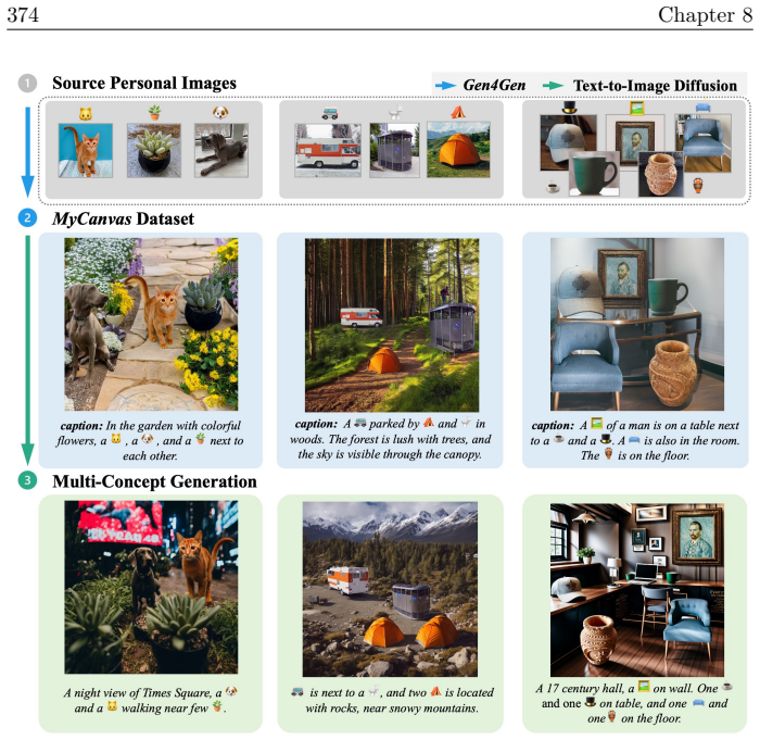
Multi-concept customization of text-to-image diffusion
[KZZ+23] Nupur Kumari, Bingliang Zhang, Richard Zhang, Eli Shechtman, and Jun-Yan Zhu. “Multi-concept customization of text-to-image diffusion” .Proceedings of the IEEE/CVF conference on computer vision and pattern recognition . 2023, pp. 1931–1941. §B.3 529 [Lab24] Black Forest Labs. FLUX. https://github.com/black-forest- labs/flux
2023
-
[53]
FLUX.1 Kontext: Flow matching for in-context image generation and edit- ing in latent space
[LBB+25] Black Forest Labs, Stephen Batifol, Andreas Blattmann, Frederic Boesel, Saksham Consul, Cyril Diagne, Tim Dockhorn, Jack En- glish, Zion English, Patrick Esser, Sumith Kulal, Kyle Lacey, Yam Levi, Cheng Li, Dominik Lorenz, Jonas Müller, Dustin Podell, Robin Rombach, Harry Saini, Axel Sauer, and Luke Smith. “FLUX.1 Kontext: Flow matching for in-co...
2025
-
[54]
The Nonlinear Statistics of High-Contrast Patches in Natural Images
[LPM03] Ann Lee, Kim Pedersen, and David Mumford. “The Nonlinear Statistics of High-Contrast Patches in Natural Images” . Interna- tional Journal of Computer Vision 54 (Aug. 2003). [LSJ+16] Jason D Lee, Max Simchowitz, Michael I Jordan, and Benjamin Recht. “Gradient descent only converges to minimizers” . Confer- ence on learning theory . PMLR. 2016, pp. ...
2003
-
[55]
O (d/T) convergence theory for diffusion probabilistic models under minimal assumptions
Proceedings of Machine Learning Research. PMLR, July 2018, pp. 2965–2974. 530 Appendix B [LY24] Gen Li and Yuling Yan. “O (d/T) convergence theory for diffusion probabilistic models under minimal assumptions” . arXiv preprint arXiv:2409.18959 (2024). [LFD+22] Haochuan Li, Farzan Farnia, Subhro Das, and Ali Jadbabaie. “On convergence of gradient descent as...
arXiv 2018
-
[56]
Repair- ing Sparse Low-Rank Texture
[LRZ+12] Xiao Liang, Xiang Ren, Zhengdong Zhang, and Yi Ma. “Repair- ing Sparse Low-Rank Texture” . Computer Vision – ECCV 2012 . Ed. by Andrew Fitzgibbon, Svetlana Lazebnik, Pietro Perona, Yoichi Sato, and Cordelia Schmid. Berlin, Heidelberg: Springer Berlin Heidelberg, 2012, pp. 482–495. [LMB+14] Tsung-Yi Lin, Michael Maire, Serge Belongie, James Hays, ...
2012
-
[57]
Multi- scale geometric methods for data sets I: Multiscale SVD, noise and curvature
[LMR17] Anna V. Little, Mauro Maggioni, and Lorenzo Rosasco. “Multi- scale geometric methods for data sets I: Multiscale SVD, noise and curvature” . Applied and Computational Harmonic Analysis 43.3 (2017), pp. 504–567. [LMZ+24] Jiacheng Liu, Sewon Min, Luke Zettlemoyer, Yejin Choi, and Hannaneh Hajishirzi. “Infini-gram: Scaling unbounded n-gram language m...
arXiv 2017
-
[58]
Decoupled Weight Decay Reg- ularization
[LH19] Ilya Loshchilov and Frank Hutter. “Decoupled Weight Decay Reg- ularization” .arXiv preprint arXiv:1711.05101 (2019). 532 Appendix B [MYP+10] M. Journée, Y. Nesterov, P. Richtárik, and R. Sepulchre. “Gen- eralized power method for sparse principal component analysis” . Journal of Machine Learning Research 11 (2010), pp. 517–553. [MDH+07a] Y. Ma, H. ...
Pith/arXiv arXiv 2019
-
[59]
Segmenta- tion of multivariate mixed data via lossy data coding and com- pression
[MDH+07b] Yi Ma, Harm Derksen, Wei Hong, and John Wright. “Segmenta- tion of multivariate mixed data via lossy data coding and com- pression” . IEEE transactions on pattern analysis and machine intelligence 29.9 (2007), pp. 1546–1562. [MHN13] Andrew L Maas, Awni Y Hannun, and Andrew Y Ng. “Recti- fier nonlinearities improve neural network acoustic models”...
2007
-
[60]
AMASS: Archive of motion capture as surface shapes
[MGT+19] Naureen Mahmood, Nima Ghorbani, Nikolaus F Troje, Gerard Pons-Moll, and Michael J Black. “AMASS: Archive of motion capture as surface shapes” .Proceedings of the IEEE/CVF Confer- ence on Computer Vision and Pattern Recognition. 2019, pp. 5442–
2019
-
[61]
Sparse Modeling for Image and Vision Processing
[MBP14] Julien Mairal, Francis Bach, and Jean Ponce. “Sparse Modeling for Image and Vision Processing” . Foundations and Trends® in Computer Graphics and Vision 8.2-3 (2014), pp. 85–283. [MSM93] Mitchell P. Marcus, Beatrice Santorini, and Mary Ann Marcinkiewicz. “Building a Large Annotated Corpus of English: The Penn T reebank” . Computational Linguistics...
arXiv 2014
-
[62]
A Proposal for the Dartmouth Summer Research Project on Artificial Intelligence: August 31, 1955
[MMR+06] John McCarthy, Marvin L. Minsky, Nathaniel Rochester, and Claude E. Shannon. “A Proposal for the Dartmouth Summer Research Project on Artificial Intelligence: August 31, 1955” . AI Mag. 27.4 (Dec. 2006), pp. 12–14. §B.3 533 [MC89] Michael McCloskey and Neal J Cohen. “Catastrophic interfer- ence in connectionist networks: The sequential learning p...
1955
-
[63]
A Logical Calculus of the Ideas Immanent in Nervous Activity
Elsevier, 1989, pp. 109–165. [MP43] Warren McCulloch and Walter Pitts. “A Logical Calculus of the Ideas Immanent in Nervous Activity” . Bulletin of Mathematical Biophysics 5 (1943), pp. 115–133. [MM70] Jerry M. Mendel and Robert W. Mclaren. “Reinforcement-learning control and pattern recognition systems” . In Mendel, J. M. and Fu, K. S., editors, Adaptive...
1989
-
[64]
Continuum percolation thresholds in two dimensions
arXiv: 1609 . 07843 [cs.CL] . [MM12] Stephan Mertens and Cristopher Moore. “Continuum percolation thresholds in two dimensions” . Phys. Rev. E 86 (6 Dec. 2012), p. 061109. [MON+19] Lars Mescheder, Michael Oechsle, Michael Niemeyer, Sebastian Nowozin, and Andreas Geiger. “Occupancy Networks: Learning 3D Reconstruction in Function Space” . 2019 IEEE/CVF Con...
arXiv 2012
-
[65]
SYMMETRIC GAUGE FUNCTIONS AND UNI- TARILY INV ARIANT NORMS
[Mir60] L Mirsky. “SYMMETRIC GAUGE FUNCTIONS AND UNI- TARILY INV ARIANT NORMS” .The Quarterly Journal of Math- ematics 11.1 (Jan. 1960), pp. 50–59. [MCS+22] Paritosh Mittal, Yen-Chi Cheng, Maneesh Singh, and Shubham Tulsiani. “Autosdf: Shape priors for 3d completion, reconstruc- tion and generation” . Proceedings of the IEEE/CVF conference on computer vis...
Pith/arXiv arXiv 1960
-
[66]
Stochastic Models for Generic Images
[MG99] David Mumford and Basilis Gidas. “Stochastic Models for Generic Images” .Quarterly of Applied Mathematics 59 (July 1999). [MK07] Joseph F Murray and Kenneth Kreutz-Delgado. “Learning sparse overcomplete codes for images” . The Journal of VLSI Signal Pro- cessing Systems for Signal Image and Video Technology 46.1 (Mar. 2007), pp. 1–13. [MLS94] R. Mu...
1999
-
[67]
The cosparse analysis model and algorithms
[NDE+13] S. Nam, M.E. Davies, M. Elad, and R. Gribonval. “The cosparse analysis model and algorithms” . Applied and Computational Har- monic Analysis 34.1 (2013), pp. 30–56. [NGE+20] Charlie Nash, Yaroslav Ganin, SM Ali Eslami, and Peter Battaglia. “Polygen: An autoregressive generative model of 3d meshes” . In- ternational conference on machine learning....
2013
-
[68]
Point-e: A system for generating 3d point clouds from complex prompts
[NJD+22] Alex Nichol, Heewoo Jun, Prafulla Dhariwal, Pamela Mishkin, and Mark Chen. “Point-e: A system for generating 3d point clouds from complex prompts” .arXiv preprint arXiv:2212.08751 (2022). [ND21] Alexander Quinn Nichol and Prafulla Dhariwal. “Improved De- noising Diffusion Probabilistic Models” . International Conference on Machine Learning (ICML)
Pith/arXiv arXiv 2022
-
[69]
Towards a Mechanistic Explanation of Diffusion Model Generalization
[NZM+24] Matthew Niedoba, Berend Zwartsenberg, Kevin Murphy, and Frank Wood. “Towards a Mechanistic Explanation of Diffusion Model Generalization” . arXiv preprint arXiv:2411.19339 (2024). [NMM19] Oliver Nina, Jamison Moody, and Clarissa Milligan. “A Decoder- Free Approach for Unsupervised Clustering and Manifold Learn- ing with Random Triplet Mining” .20...
arXiv 2024
-
[70]
Activation functions: Comparison of trends in practice and research for deep learning
[NIG+18] Chigozie Nwankpa, Winifred Ijomah, Anthony Gachagan, and Stephen Marshall. “Activation functions: Comparison of trends in practice and research for deep learning” .arXiv preprint arXiv:1811.03378 (2018). [Oja82] Erkki Oja. “A simplified neuron model as a principal component analyzer” .Journal of Mathematical Biology 15 (1982), pp. 267–
Pith/arXiv arXiv 2018
-
[71]
A statis- tical theory of contrastive pre-training and multimodal generative AI
[OLC+25] Kazusato Oko, Licong Lin, Yuhang Cai, and Song Mei. “A statis- tical theory of contrastive pre-training and multimodal generative AI” .arXiv [cs.LG] (Jan. 2025). arXiv: 2501.04641 [cs.LG] . [OF97] B A Olshausen and D J Field. “Sparse coding with an overcom- plete basis set: a strategy employed by V1?” Vision research 37.23 (Dec. 1997), pp. 3311–3...
arXiv 2025
-
[72]
Representa- tion Learning with Contrastive Predictive Coding
[OL V18] Aaron van den Oord, Yazhe Li, and Oriol Vinyals. “Representa- tion Learning with Contrastive Predictive Coding” . arXiv [cs.LG] (July 2018). arXiv: 1807.03748 [cs.LG] . [OVK17] Aaron van den Oord, Oriol Vinyals, and Koray Kavukcuoglu. “Neural discrete representation learning” . arXiv [cs.LG] (Nov. 2017). arXiv: 1711.00937 [cs.LG] . [Ope24] OpenAI...
Pith/arXiv arXiv 2018
-
[73]
Dinov2: Learn- ing robust visual features without supervision
536 Appendix B [ODM+23] Maxime Oquab, Timothée Darcet, Théo Moutakanni, Huy Vo, Marc Szafraniec, Vasil Khalidov, Pierre Fernandez, Daniel Haz- iza, Francisco Massa, Alaaeldin El-Nouby, et al. “Dinov2: Learn- ing robust visual features without supervision” . arXiv preprint arXiv:2304.07193 (2023). [ODM+24] Maxime Oquab, Timothée Darcet, Théo Moutakanni, Hu...
Pith/arXiv arXiv 2023
-
[74]
Pursuit of a discriminative representa- tion for multiple subspaces via sequential games
[PPC+23] Druv Pai, Michael Psenka, Chih-Yuan Chiu, Manxi Wu, Edgar Dobriban, and Yi Ma. “Pursuit of a discriminative representa- tion for multiple subspaces via sequential games” . Journal of the Franklin Institute 360.6 (2023), pp. 4135–4171. [PCY+23] Xiaqing Pan, Nicholas Charron, Yongqian Yang, Scott Peters, Thomas Whelan, Chen Kong, Omkar Parkhi, Rich...
2023
-
[75]
Prevalence of Neural Collapse during the terminal phase of deep learning train- ing
arXiv: 1606.06031 [cs.CL] . [PHD20] Vardan Papyan, XY Han, and David L Donoho. “Prevalence of Neural Collapse during the terminal phase of deep learning train- ing” .arXiv preprint arXiv:2008.08186 (2020). [PRE17] Vardan Papyan, Yaniv Romano, and Michael Elad. “Convolu- tional neural networks analyzed via convolutional sparse coding” . The Journal of Mach...
Pith/arXiv arXiv 2008
-
[76]
The Linear Rep- resentation Hypothesis and the Geometry of Large Language Models
[PCV24] Kiho Park, Yo Joong Choe, and Victor Veitch. “The Linear Rep- resentation Hypothesis and the Geometry of Large Language Models” .International Conference on Machine Learning . PMLR. 2024, pp. 39643–39666. §B.3 537 [Par04] Andrew Parker. In The Blink Of An Eye: How Vision Sparked The Big Bang Of Evolution . Basic Books,
2024
-
[77]
On Lines and Planes of Closest Fit to Systems of Points in Space
[Pea01] K. Pearson. “On Lines and Planes of Closest Fit to Systems of Points in Space” .Philosophical Magazine 2.6 (1901), pp. 559–572. [PX23] William Peebles and Saining Xie. “Scalable diffusion models with transformers” .Proceedings of the IEEE/CVF international con- ference on computer vision . 2023, pp. 4195–4205. [PV25] Liangzu Peng and René Vidal. “...
arXiv 1901
-
[78]
A self-supervised descriptor for im- age copy detection
[PRR+22] Ed Pizzi, Sreya Dutta Roy, Sugosh Nagavara Ravindra, Priya Goyal, and Matthijs Douze. “A self-supervised descriptor for im- age copy detection” . Proceedings of the IEEE/CVF Conference on Computer Vision and Pattern Recognition . 2022, pp. 14532– 14542. [Pla99] S. E. Plamer. Vision Science: Photons to Phenomenology . The MIT Press,
2022
-
[79]
Sdxl: Improving latent diffusion models for high-resolution im- age synthesis
[PEL+23] Dustin Podell, Zion English, Kyle Lacey, Andreas Blattmann, Tim Dockhorn, Jonas Müller, Joe Penna, and Robin Rombach. “Sdxl: Improving latent diffusion models for high-resolution im- age synthesis” .arXiv preprint arXiv:2307.01952 (2023). [PW22] Yuri Poliyanski and Yihong Wu. Information Theory: From Cod- ing to Learning . Cambridge University Press,
Pith/arXiv arXiv 2023
-
[80]
Representation Learning via Manifold Flattening and Reconstruction
[PPR+24] Michael Psenka, Druv Pai, Vishal Raman, Shankar Sastry, and Yi Ma. “Representation Learning via Manifold Flattening and Reconstruction” .Journal of Machine Learning Research 25.132 (2024), pp. 1–47. 538 Appendix B [QSM+17] Charles R Qi, Hao Su, Kaichun Mo, and Leonidas J Guibas. “Pointnet: Deep learning on point sets for 3d classification and seg...
2024
discussion (0)
Sign in with ORCID, Apple, or X to comment. Anyone can read and Pith papers without signing in.