REVIEW 4 major objections 6 minor 50 references
Modeling Continuous Spatial-temporal Dynamics of Turbulent Flow with Test-time Refinement
T0 review · 4 major / 6 minor · reviewed 2026-08-10 · deepseek-v4-flash
Pith's one-line read Test-time refinement reconstructs DNS fields from LES with top accuracy
desk verdict A competent incremental paper with a real test-time refinement idea, but the kinetic-energy validation is partly circular and needs an ablation to show the constraint's actual contribution. read the letter →
The pith
A machine-rendered reading of the paper's core claim, the machinery that carries it, and where it could break.
The reading
What carries the argument
The load-bearing machinery is the Continuous Spatial Transition Unit (CSTU) plus a test-time refinement loop. CSTU combines the physics-guided recurrent unit (PRU), which advances the velocity field with a Runge-Kutta scheme whose temporal derivatives come from the incompressible Navier-Stokes equation, with an implicit neural representation (INR) that resamples the field onto arbitrary query points. The refinement loop uses a degradation operator that downsamples the reconstructed DNS to the LES grid and then adjusts the network's last layer at every test step to reduce the loss $L_{\text{refine}} = \alpha_0 L_{\text{deg}} + \alpha_1 L_{\text{mean}} + \alpha_2 L_{\text{kinetic}}$, where $L_{\text{deg}}$ is the mismatch with LES, $L_{\text{mean}}$ enforces equal mean velocity, and $L_{\text{kinetic}}$ pushes total kinetic energy toward a value extrapolated from the training DNS.
What would settle it
Run the trained model on a turbulent flow whose forcing varies in time or that undergoes transition, so that total kinetic energy rises or oscillates rather than staying constant or decaying linearly; if the test-time refinement then pulls reconstructions toward the wrong energy level and the SSIM or dissipation advantage over unrefined CSTU disappears, the central claim that LES-based refinement is the source of the gain is contradicted.
Extended reading notes
Core claim
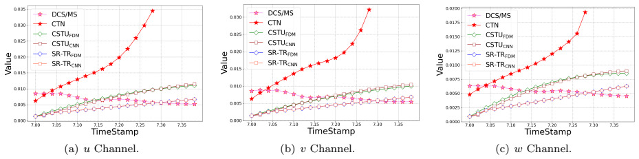
The discovery the paper argues for is that low-resolution LES data, used only at test time, are enough to stabilize learned DNS reconstruction: instead of training the network to map LES to DNS, one trains a sequential predictor on DNS alone and then, during forecasting, downsamples each reconstructed DNS field with a fixed degradation operator, compares it to the observed LES field, and updates the last layer of the model to minimize a weighted combination of the degradation loss, a mean-field loss, and a kinetic-energy loss. The reported result is that this refinement raises SSIM from about 0.936 to 0.949 on forced isotropic turbulence and from about 0.705 to 0.918 on Taylor-Green vortex data over the first ten test steps, while also lowering dissipation difference, and that it prevents the late-time error growth seen in unrefined CSTU baselines.
Load-bearing premise
The refinement assumes the total kinetic energy of the test flow follows the same simple time pattern (constant or linearly decaying) as the training period, because that pattern is extrapolated and enforced as a hard penalty rather than derived from the governing equations.
Editorial extensions
If this is right
- Reconstructing DNS from LES no longer requires paired high-resolution data at test time, only the cheap LES stream and a short training-period DNS history.
- The refinement loss can be attached to other sequential predictors, since it only adjusts the last layer and needs no architectural change.
- One trained model can be applied zero-shot at target resolutions above the training resolution, with optional fine-tuning on a few high-resolution DNS samples improving it further.
- Long-horizon forecasting of turbulent fields becomes more stable, since the degradation loop prevents cumulative error growth in the velocity and kinetic-energy statistics.
- Using LES as an additional input brings little benefit once the test-time refinement is in place, so the cheap LES stream is best spent as a constraint rather than a feature.
Reading between the lines
- Editorial inference: the same degradation-based refinement idea could work for other under-resolved simulations paired with coarse observations, such as ocean or climate models, wherever a coarse, frequently available field can serve as an anchor.
- Editorial inference: the paper's framing suggests a testable extension where the kinetic-energy prior is replaced by an online estimator built from the LES stream itself, which would remove the main assumption of stationary or linearly decaying energy.
- Editorial inference: because refinement only tunes the last layer, it could be run in an online or streaming setting, adapting the reconstruction as new LES frames arrive without retraining.
- Editorial inference: the zero-shot multi-resolution results imply the INR learns a quasi-continuous spatial representation of the flow, so probing the model at arbitrary off-grid points, not just coarse and fine grids, is a direct way to test how continuous that representation really is.
Editorial analysis
A structured set of objections, weighed in public.
Referee Report
Summary. The paper proposes SR-TR (Super-Resolution through Test-time Refinement), a physics-guided neural network for reconstructing high-resolution DNS fields from lower-resolution LES data in unsteady incompressible turbulent flows. The method combines a physics-guided recurrent unit (PRU) based on a Runge-Kutta discretization of the Navier-Stokes equations with a continuous spatial transition unit (CSTU) based on implicit neural representations, enabling prediction at arbitrary resolutions. During testing, the reconstructed DNS is refined by minimizing a loss that includes a degradation term against available LES data, an equal-mean constraint, and a kinetic-energy constraint. The authors evaluate SR-TR on forced isotropic turbulence and Taylor-Green vortex flows, reporting higher SSIM and lower dissipation difference than several super-resolution, downscaling, and neural-operator baselines, as well as improved long-term behavior over 20 forecast steps. The implementation is stated to be publicly available.
Significance. The central idea of using LES data at test time through a degradation-based refinement, rather than as a training input, is valuable and potentially of broad interest for turbulence reconstruction and for other PDE-constrained super-resolution tasks. The CSTU's combination of implicit neural representation with a physics-guided recurrent unit is a sensible way to address resolution generalization, and the quantitative comparisons cover a reasonable set of baselines. The paper also ships a public implementation, which is a concrete strength. The significance of the results is currently tempered by three issues: the kinetic-energy validation is partly circular because Lkinetic directly enforces the metric used for validation; the CSTU is described as operating on 2D slices despite the 3D Navier-Stokes constraint; and the empirical tables lack error bars and contain at least one internal inconsistency. With these points addressed, the contribution would be a useful step toward physically consistent, test-time-adaptable super-resolution for turbulent flows.
major comments (4)
- [Sec. 3.1, Eq. (3.4); Sec. 4.2.3, Figs. 7 and 15] The kinetic-energy term Lkinetic is a fitted prior, and the validation in Sec. 4.2.3 uses the same quantity as a success metric. Since Eq. (3.4) directly minimizes |K(Q_d_hat) - K_tilde|, the agreement between reconstructed and DNS kinetic energy in Figs. 7 and 15 is achieved partly by construction rather than by the model's predictive ability. Both test flows are in the favorable regime for this prior: forced isotropic turbulence has stationary kinetic energy and the Taylor-Green vortex decays monotonically. The paper reports no ablation with Lkinetic removed, so it is unknown whether the claimed long-term stability is due to the physical constraint or merely to the enforced energy level. Please add such an ablation, report SSIM and dissipation difference for that variant, and test at least one out-of-favorable-regime case (e.g., time-varying forcing or transition), or explicitly limit the claim to flows with stationary or linearly decaying energy.
- [Sec. 3.2, Eqs. (3.6)-(3.7); Sec. 2.1, Eq. (2.1)] The CSTU is described as operating on "each flow data slice" in a continuous 2D feature space, but the physics constraint is the 3D Navier-Stokes equation in Eq. (2.1). If the PRU estimates spatial derivatives only in the x-y plane, the z-gradient terms are omitted and the model does not enforce the full incompressible Navier-Stokes dynamics on which the physical-consistency claim rests. Please state explicitly how the z-direction is handled, whether adjacent slices are coupled in the gradient computation, and, if gradients are only two-dimensional, provide results with full 3D gradient computation or explain why the omission does not affect the central conclusions.
- [Table 1] The reported SSIM for SRGAN in the w channel is 0.215, while the u and v channels are 0.891 and 0.881, and all other entries in the table are above 0.6. This is almost certainly a typographical error, but it makes the table internally inconsistent and undermines the quantitative comparison. Please correct the entry and verify all reported numbers in Tables 1 and 2.
- [Sec. 4.1.3, Tables 1 and 2] All quantitative results are reported as averages over the first 10 time steps, without error bars, confidence intervals, or the number of random seeds. Some of the reported differences between SR-TR and the strongest baselines are small (e.g., SSIM 0.949 vs 0.936 for SR-TR FDM vs CSTU FDM in Table 1), so the observed ranking could change with statistical variability. Please provide variance estimates or per-seed results so the reader can assess the significance of the improvements.
minor comments (6)
- [Appendix A.2, Sec. 4.1.2] The method is named SR-TR, but the appendix and parts of the text refer to "ST-TR FDM" and "ST-TR CNN"; please unify the notation.
- [Sec. 3.2] The text contains the misspelling "Runga-Kutta" and should read "Runge-Kutta."
- [Sec. 4.1.3, Ref. [48]] The dissipation metric is attributed to a Wikipedia article on the Laplace operator; please cite a standard fluid-dynamics reference for dissipation or pseudo-dissipation instead.
- [Sec. 3.1, Eq. (3.3)] The equal-mean loss is written as Lmean = |Q_l - Q_d_hat|, but comparing the full LES field with the reconstructed DNS field is ambiguous because the fields have different resolutions; clarify whether the mean is taken over spatial dimensions and whether Q_l is upsampled or Q_d_hat is downsampled before the difference is computed.
- [Abstract, Sec. 3.1, Sec. 3.2] The abstract states that LES data are used "only in the testing phase," but Sec. 3.2 introduces a variant that uses LES data as additional input during prediction and presumably during training; please state more precisely that LES data are used only at test time in the core SR-TR variant, while an optional variant incorporates LES as input.
- [Sec. 4.2.4, Fig. 8] The notation "SR-TR_f FDM" is introduced in the text but the figure caption is compressed and unclear; please spell out the subscript in the figure and caption.
Circularity Check
Kinetic-energy validation in Sec. 4.2.3 is partly circular because Eq. (3.4) directly optimizes the same quantity used as the validation metric; SSIM and dissipation results remain independent.
-
fitted input called prediction
[Eq. (3.4) and Sec. 4.2.3 (Validation via physical metrics)]
"However, the value of kinetic energy for incompressible flows often follows simple patterns, e.g., constant or linearly decayed, and thus can be approximated from the DNS data in the training period, denoted by ˜K. Therefore, the loss function Lkinetic is defined as follows: (3.4) Lkinetic = |K( ˆQ d ) − ˜K|. ... The performance is also evaluated through the long-term prediction of turbulent kinetic energy. Figure 7 illustrates the energies corresponding to the target DNS, along with the reconstructed flow data from both the baselines and SR-TR-based methods for the FIT dataset."
The test-time refinement minimizes Lkinetic at every refinement step, explicitly driving K(Qhat_d) toward Ktilde, a value extrapolated from training-period DNS. For FIT and TGV, Ktilde is deliberately chosen to match the test-period DNS energy because the energy is stationary or monotonically decaying. Therefore, the Sec. 4.2.3 demonstration that SR-TR tracks DNS kinetic energy is not an independent check: it is the optimization objective itself, provided Ktilde is a good extrapolation. The SSIM and dissipation-difference results are independent, but the kinetic-energy evidence for 'preserving physical attributes' is forced by construction.
full rationale
The paper's main quantitative evaluation against held-out DNS is not circular: SSIM and dissipation difference are computed on testing-period data and are not part of any training or refinement loss. The PRU self-citation [41] is also not load-bearing evidence; PRU is used as an architectural component, not as a justification for the paper's claims. The circularity is localized to the kinetic-energy validation. Eq. (3.4) defines a refinement loss minimizing |K(Qhat_d) - Ktilde|, and Sec. 4.2.3/Fig. 7 then uses closeness of K(Qhat_d) to DNS kinetic energy as evidence of success. Since Ktilde is extrapolated from DNS training data and the tested flows are exactly those where the constant/linear-decay energy assumption holds, the SR-TR kinetic-energy curves are close by construction. This does not invalidate the independent SSIM and dissipation results, but it does make the physical-attribute claim based on kinetic energy partly circular. Score is set to 6 rather than higher because the central reconstruction claim still rests on held-out, non-loss metrics; the circularity is partial and confined to one validation channel.
Assumptions & free parameters
free parameters (3)
- PRU Runge-Kutta weights {w_n} =
not listed
- Refinement loss weights alpha0, alpha1, alpha2 =
1000, 1, 1
- Kinetic energy target K~ =
constant or linearly decaying function
assumptions (5)
- domain assumption Incompressible Newtonian flow with constant density
- domain assumption LES data are consistent with a downsampled DNS field
- ad hoc to paper Kinetic energy of the test flow follows the same simple pattern as training DNS
- domain assumption Boundary conditions are periodic
- ad hoc to paper The CSTU operates on 2D slices and omits z-gradients in the Navier-Stokes constraint
Cite this review
Pith. "Pith review of Modeling Continuous Spatial-temporal Dynamics of Turbulent Flow with Test-time Refinement." pith.science (2026). https://pith.science/paper/V4JQQQPC
@misc{pith2026241219927,
  author       = {Pith},
  title        = {Pith review of: Modeling Continuous Spatial-temporal Dynamics of Turbulent Flow with Test-time Refinement},
  year         = {2026},
  howpublished = {\url{https://pith.science/paper/V4JQQQPC}},
  note         = {Machine review of arXiv:2412.19927}
}
read the original abstract
The precise simulation of turbulent flows holds immense significance across various scientific and engineering domains, including climate science, freshwater science, and energy-efficient manufacturing. Within the realm of simulating turbulent flows, large eddy simulation (LES) has emerged as a prevalent alternative to direct numerical simulation (DNS), offering computational efficiency. However, LES cannot accurately capture the full spectrum of turbulent transport scales and is present only at a lower spatial resolution. Reconstructing high-fidelity DNS data from the lower-resolution LES data is essential for numerous applications, but it poses significant challenges to existing super-resolution techniques, primarily due to the complex spatio-temporal nature of turbulent flows. This paper proposes a novel flow reconstruction approach that leverages physical knowledge to model flow dynamics. Different from traditional super-resolution techniques, the proposed approach uses LES data only in the testing phase through a degradation-based refinement approach to enforce physical constraints and mitigate cumulative reconstruction errors over time. Furthermore, a feature sampling strategy is developed to enable flow data reconstruction across different resolutions. The results on two distinct sets of turbulent flow data indicate the effectiveness of the proposed method in reconstructing high-resolution DNS data, preserving the inherent physical attributes of flow transport, and achieving DNS reconstruction at different resolutions.
Figures


Figures from the paper (13 more)






Reference graph
Works this paper leans on
-
[1]
Gulf stream shifts following enso events
Arnold H Taylor, Michael B Jordan, and John A Stephens. Gulf stream shifts following enso events. Nature, 393(6686):638–638, 1998
work page 1998
- [2]
-
[3]
K Qu, HS Tang, and A Agrawal. Integration of fully 3d fluid dynamics and geophysical fluid dynamics models for multiphysics coastal ocean flows: Simulation of lo- cal complex free-surface phenomena. Ocean Modelling, 135:14–30, 2019
work page 2019
-
[4]
Deep learning to represent subgrid processes in climate models
Stephan Rasp, Michael S Pritchard, and Pierre Gen- tine. Deep learning to represent subgrid processes in climate models. Proceedings of the National Academy of Sciences, 2018
work page 2018
-
[5]
P. Givi. Spectral and random vortex methods in turbulent reacting flows. In P. A. Libby and F. A. Williams, editors, Turbulent Reacting Flows, chapter 8, pages 475–572. Academic Press, London, England, 1994
work page 1994
-
[6]
Large eddy simulation for incompress- ible flows: an introduction
Pierre Sagaut. Large eddy simulation for incompress- ible flows: an introduction . Springer Science & Busi- ness Media, 2005
work page 2005
-
[7]
Self-contained filtered density function
Arash G Nouri, Mehdi B Nik, Pope Givi, Daniel Livescu, and Stephen B Pope. Self-contained filtered density function. Physical Review Fluids , 2(9):094603, 2017
work page 2017
-
[8]
Super-resolution image reconstruction: a technical overview
Sung Cheol Park, Min Kyu Park, and Moon Gi Kang. Super-resolution image reconstruction: a technical overview. IEEE signal processing magazine , 20(3):21– 36, 2003
work page 2003
Show all 50 references
-
[9]
Understanding of a convolutional neural net- work
Saad Albawi, Tareq Abed Mohammed, and Saad Al- Zawi. Understanding of a convolutional neural net- work. In 2017 international conference on engineering and technology (ICET) , pages 1–6. IEEE, 2017
2017
-
[10]
Learning a deep convolutional network for image super-resolution
Chao Dong, Chen Change Loy, Kaiming He, and Xi- aoou Tang. Learning a deep convolutional network for image super-resolution. In Computer Vision–ECCV 2014: 13th European Conference, Zurich, Switzerland, September 6-12, 2014, Proceedings, Part IV 13 , pages 184–199. Springer, 2014
2014
-
[11]
Residual dense network for image super- resolution
Yulun Zhang, Yapeng Tian, Yu Kong, Bineng Zhong, and Yun Fu. Residual dense network for image super- resolution. arXiv preprint arXiv:1802.08797 , 2018
2018 arXiv
-
[12]
Fast, accurate, and lightweight super-resolution with cascading residual network
Namhyuk Ahn, Byungkon Kang, and Kyung-Ah Sohn. Fast, accurate, and lightweight super-resolution with cascading residual network. In Proceedings of the Eu- ropean conference on computer vision (ECCV) , pages 252–268, 2018
2018
-
[13]
Second-order attention network for sin- gle image super-resolution
Tao Dai, Jianrui Cai, Yongbing Zhang, Shu-Tao Xia, and Lei Zhang. Second-order attention network for sin- gle image super-resolution. In 2019 IEEE/CVF Con- ference on Computer Vision and Pattern Recognition (CVPR), pages 11057–11066, 2019
2019
-
[14]
A fast and efficient super- resolution network using hierarchical dense residual learning
Vinh Van Duong, Thuc Nguyen Huu, Jonghoon Yim, and Byeungwoo Jeon. A fast and efficient super- resolution network using hierarchical dense residual learning. In 2021 IEEE International Conference on Image Processing (ICIP) , pages 1809–1813. IEEE, 2021
2021
-
[15]
Image super-resolution using very deep residual channel attention networks
Yulun Zhang, Kunpeng Li, Kai Li, Lichen Wang, Bineng Zhong, and Yun Fu. Image super-resolution using very deep residual channel attention networks. In Proceedings of the European conference on computer vision (ECCV) , pages 286–301, 2018
2018
-
[16]
Photo-realistic single image super- resolution using a generative adversarial network
Christian Ledig, Lucas Theis, Ferenc Husz´ ar, Jose Caballero, Andrew Cunningham, Alejandro Acosta, Andrew Aitken, Alykhan Tejani, Johannes Totz, Ze- han Wang, et al. Photo-realistic single image super- resolution using a generative adversarial network. In Proceedings of the I...
2017
-
[17]
Recovering realistic texture in image super- resolution by deep spatial feature transform
Xintao Wang, Ke Yu, Chao Dong, and Chen Change Loy. Recovering realistic texture in image super- resolution by deep spatial feature transform. In Pro- ceedings of the IEEE conference on computer vision and pattern recognition, pages 606–615, 2018
2018
-
[18]
Esr- gan: Enhanced super-resolution generative adversarial networks
Xintao Wang, Ke Yu, Shixiang Wu, Jinjin Gu, Yihao Liu, Chao Dong, Yu Qiao, and Chen Change Loy. Esr- gan: Enhanced super-resolution generative adversarial networks. In ECCV Workshops , 2018
2018
-
[19]
Progressive growing of gans for improved quality, stability, and variation
Tero Karras, Timo Aila, Samuli Laine, and Jaakko Lehtinen. Progressive growing of gans for improved quality, stability, and variation. arXiv preprint arXiv:1710.10196, 2017
2017 arXiv
-
[20]
Robust super-resolution gan, with manifold-based and percep- tion loss
Uddeshya Upadhyay and Suyash P Awate. Robust super-resolution gan, with manifold-based and percep- tion loss. In 2019 IEEE 16th International Symposium on Biomedical Imaging (ISBI 2019) . IEEE, 2019
2019
-
[21]
Mfagan: A compression framework for memory-efficient on-device super-resolution gan
Wenlong Cheng, Mingbo Zhao, Zhiling Ye, and Shuhang Gu. Mfagan: A compression framework for memory-efficient on-device super-resolution gan. arXiv preprint arXiv:2107.12679, 2021
2021 arXiv
-
[22]
Ranksrgan: Generative adversarial networks with ranker for image super-resolution
Zhang Wenlong, Liu Yihao, Chao Dong, and Yu Qiao. Ranksrgan: Generative adversarial networks with ranker for image super-resolution. IEEE Transac- tions on Pattern Analysis and Machine Intelligence , 44(10):1–1, 2021
2021
-
[23]
Adversarial generation of continuous im- ages
Ivan Skorokhodov, Savva Ignatyev, and Mohamed El- hoseiny. Adversarial generation of continuous im- ages. In Proceedings of the IEEE/CVF conference on computer vision and pattern recognition , pages 10753– 10764, 2021
2021
-
[24]
Learning Copyright © 2025 by SIAM Unauthorized reproduction of this article is prohibited continuous image representation with local implicit image function
Yinbo Chen, Sifei Liu, and Xiaolong Wang. Learning Copyright © 2025 by SIAM Unauthorized reproduction of this article is prohibited continuous image representation with local implicit image function. In Proceedings of the IEEE/CVF conference on computer vision and pattern reco...
2025
-
[25]
Magnet: Mesh agnostic neural pde solver
Oussama Boussif, Yoshua Bengio, Loubna Benabbou, and Dan Assouline. Magnet: Mesh agnostic neural pde solver. Advances in Neural Information Processing Systems, 35:31972–31985, 2022
2022
-
[26]
Videoinr: Learning video implicit neural representation for continuous space-time super- resolution
Zeyuan Chen, Yinbo Chen, Jingwen Liu, Xingqian Xu, Vidit Goel, Zhangyang Wang, Humphrey Shi, and Xiaolong Wang. Videoinr: Learning video implicit neural representation for continuous space-time super- resolution. In Proceedings of the IEEE/CVF Con- ference on Computer Vision a...
2022
-
[27]
Cross- modality high-frequency transformer for mr image super-resolution
Chaowei Fang, Dingwen Zhang, Liang Wang, Yu- lun Zhang, Lechao Cheng, and Junwei Han. Cross- modality high-frequency transformer for mr image super-resolution. In Proceedings of the 30th ACM In- ternational Conference on Multimedia , pages 1584– 1592, 2022
2022
-
[28]
Transformer for single image super-resolution
Zhisheng Lu, Juncheng Li, Hong Liu, Chaoyan Huang, Linlin Zhang, and Tieyong Zeng. Transformer for single image super-resolution. In Proceedings of the IEEE/CVF conference on computer vision and pattern recognition, pages 457–466, 2022
2022
-
[29]
A hybrid network of cnn and transformer for lightweight image super-resolution
Jinsheng Fang, Hanjiang Lin, Xinyu Chen, and Kun Zeng. A hybrid network of cnn and transformer for lightweight image super-resolution. In Proceedings of the IEEE/CVF conference on computer vision and pattern recognition, pages 1103–1112, 2022
2022
-
[30]
Detail-preserving transformer for light field image super-resolution
Shunzhou Wang, Tianfei Zhou, Yao Lu, and Huijun Di. Detail-preserving transformer for light field image super-resolution. In Proceedings of the AAAI Confer- ence on Artificial Intelligence , volume 36, pages 2522– 2530, 2022
2022
-
[31]
Self-calibrated efficient trans- former for lightweight super-resolution
Wenbin Zou, Tian Ye, Weixin Zheng, Yunchen Zhang, Liang Chen, and Yi Wu. Self-calibrated efficient trans- former for lightweight super-resolution. In Proceedings of the IEEE/CVF Conference on Computer Vision and Pattern Recognition, pages 930–939, 2022
2022
-
[32]
Light field image super-resolution with transformers
Zhengyu Liang, Yingqian Wang, Longguang Wang, Jungang Yang, and Shilin Zhou. Light field image super-resolution with transformers. IEEE Signal Pro- cessing Letters, 29:563–567, 2022
2022
-
[33]
Super-resolution reconstruction of turbulent flows with machine learning
Kai Fukami, Koji Fukagata, and Kunihiko Taira. Super-resolution reconstruction of turbulent flows with machine learning. Journal of Fluid Mechanics , 870:106–120, 2019
2019
-
[34]
Machine-learning-based spatio-temporal super resolu- tion reconstruction of turbulent flows
Kai Fukami, Koji Fukagata, and Kunihiko Taira. Machine-learning-based spatio-temporal super resolu- tion reconstruction of turbulent flows. Journal of Fluid Mechanics, 2021
2021
-
[35]
Deep learning methods for super-resolution re- construction of turbulent flows
Bo Liu, Jiupeng Tang, Haibo Huang, and Xi-Yun Lu. Deep learning methods for super-resolution re- construction of turbulent flows. Physics of Fluids , 32(2):025105, 2020
2020
-
[36]
Super-resolution reconstruction of turbulent velocity fields using a generative adver- sarial network-based artificial intelligence framework
Zhiwen Deng, Chuangxin He, Yingzheng Liu, and Kyung Chun Kim. Super-resolution reconstruction of turbulent velocity fields using a generative adver- sarial network-based artificial intelligence framework. Physics of Fluids , 31(12):125111, 2019
2019
-
[37]
Super-resolution reconstruction for the three-dimensional turbulence flows with a back- projection network
Zhen Yang et al. Super-resolution reconstruction for the three-dimensional turbulence flows with a back- projection network. Physics of Fluids , 35(5), 2023
2023
-
[38]
Super-resolution reconstruction of turbulent flows with a transformer-based deep learning framework
Qin Xu et al. Super-resolution reconstruction of turbulent flows with a transformer-based deep learning framework. Physics of Fluids , 2023
2023
-
[39]
Fourier neural operator for parametric partial differential equations
Zongyi Li, Nikola Kovachki, Kamyar Azizzadenesheli, Burigede Liu, Kaushik Bhattacharya, Andrew Stuart, and Anima Anandkumar. Fourier neural operator for parametric partial differential equations. arXiv preprint arXiv:2010.08895, 2020
2010 arXiv
-
[40]
Multi-scale message passing neural pde solvers
L´ eonard Equer, T Konstantin Rusch, and Siddhartha Mishra. Multi-scale message passing neural pde solvers. arXiv preprint arXiv:2302.03580 , 2023
2023 arXiv
-
[41]
Physics guided neural networks for spatio-temporal super- resolution of turbulent flows
Tianshu Bao, Shengyu Chen, Taylor T Johnson, Pey- man Givi, Shervin Sammak, and Xiaowei Jia. Physics guided neural networks for spatio-temporal super- resolution of turbulent flows. In The 38th Conference on Uncertainty in Artificial Intelligence , 2022
2022
-
[42]
Forced isotropic turbulence data set (extended)
Wan Minping, Shiyi Chen, Gregory Eyink, Charles Meneveau, Perry Johnson, Eric Perlman, Randal Burns, Yi Li, Alex Szalay, and Stephen Hamilton. Forced isotropic turbulence data set (extended). 2012
2012
-
[43]
The taylor-green vortex and fully developed turbulence
Marc E Brachet, D Meiron, S Orszag, B Nickel, R Morf, and Uriel Frisch. The taylor-green vortex and fully developed turbulence. Journal of Statistical Physics , 34(5):1049–1063, 1984
1984
-
[44]
Runge-kutta methods
John Butcher. Runge-kutta methods. Scholarpedia, 2(9):3147, 2007
2007
-
[45]
Numerical partial differen- tial equations: finite difference methods , volume 22
James William Thomas. Numerical partial differen- tial equations: finite difference methods , volume 22. Springer Science & Business Media, 2013
2013
-
[46]
Long short- term memory
Sepp Hochreiter and J¨ urgen Schmidhuber. Long short- term memory. Neural computation , 9(8):1735–1780, 1997
1997
-
[47]
Image quality assessment: from error visibility to structural similarity
Zhou Wang, Alan C Bovik, Hamid R Sheikh, and Eero P Simoncelli. Image quality assessment: from error visibility to structural similarity. IEEE transac- tions on image processing , 13(4):600–612, 2004
2004
-
[48]
Laplace operator — Wikipedia, the free encyclopedia, 2022
Wikipedia contributors. Laplace operator — Wikipedia, the free encyclopedia, 2022. [Online; ac- cessed 23-January-2023]
2022
-
[49]
zero- shot
Assaf Shocher, Nadav Cohen, and Michal Irani. “zero- shot” super-resolution using deep internal learning. In Proceedings of the IEEE conference on computer vision and pattern recognition, pages 3118–3126, 2018
2018
-
[50]
Adam: A method for stochastic optimization
Diederik P Kingma and Jimmy Ba. Adam: A method for stochastic optimization. arXiv preprint arXiv:1412.6980, 2014. Copyright © 2025 by SIAM Unauthorized reproduction of this article is prohibited A Experimental Settings A.1 Dataset To evaluate the performance of the proposed me...
2014 arXiv
Reviewed August 10, 2026 · model on record in the stance chip above.
Discussion (0). Continue with ORCID to comment.