REVIEW 4 major objections 5 minor 45 references
A parameter-free closure reproduces the decay laws and mixing constants of decaying isotropic turbulence.
Reviewed by Pith at T0; open to challenge. T0 means a machine referee read the full paper against a public rubric. the ladder, T0–T4 →
T0 review · deepseek-v4-flash
2026-08-01 05:46 UTC pith:V4UYHFD2
load-bearing objection A self-consistent closure framework, but the validation claim outruns the evidence: the core identity (7) is never tested against independent data. the 4 major comments →
Numerical Validation of Lyapunov-Liouville Theory and Non-Diffusive Closures in Decaying Isotropic Fluid and Scalar Turbulence
The pith
A machine-rendered reading of the paper's core claim, the machinery that carries it, and where it could break.
Core claim
On the author's own terms, the central discovery is that the non-diffusive closures K = u^3 sqrt((1−f)/2) ∂f/∂r and G = u θ^2 sqrt((1−f)/2) ∂fθ/∂r, derived from the link ⟨Λ_L²(r)⟩_L r² = 2u²(1−f) between the finite-scale Lagrangian Lyapunov exponent and the longitudinal velocity correlation, close the von Kármán–Howarth and Corrsin equations. Numerical integration of the closed system from Saffman–Birkhoff, Loitsiansky, and Gaussian initial conditions reproduces the empirically known decay exponents for each case, the Kolmogorov and Yaglom functions peaking near 4/5 and 2/3, the spectral constants C_B ≃ 3.5 and C_OC ≃ 1.8, and the growth of small-scale intermittency in temperature increments
What carries the argument
The load-bearing link is Eq. (7): the mean-square finite-scale Lagrangian Lyapunov exponent times the squared separation equals twice the velocity variance times (1 − f(r)). Combined with the spectral-gap hierarchy (1) separating Lagrangian from Eulerian fluctuation rates, this yields algebraic closures (6) for the triple correlations in terms of the double correlations only. These closures fix the small-scale skewness to −3/7, the Rλ = 10 validity threshold, and the parametric family of increment PDFs via the characteristic function χ(Rλ).
Load-bearing premise
The entire validation rests on Eq. (7), the asserted proportionality between the squared finite-scale Lagrangian Lyapunov exponent and the correlation defect 2u²(1−f); the paper neither derives it in this work nor tests it directly against DNS or experiments, so if that link is wrong the closure (6) and all resulting exponents and constants are a self-consistent simulation of a false premise.
What would settle it
A direct numerical simulation of forced or freely decaying HIT that computes both sides of Eq. (7) across the inertial range, or that compares the simulated triple correlation k(r) with the closure value u³√((1−f)/2) ∂f/∂r. A systematic disagreement at moderate Reynolds numbers would invalidate the premise; agreement would strongly support the closed system.
If this is right
- If the closure stands, the decay exponents of freely decaying homogeneous isotropic turbulence are not universal but follow directly from the initial correlation profile, matching Saffman–Birkhoff and Loitsiansky classes without ad hoc constants.
- The 4/5-law and 2/3-law maxima in decaying flows are obtained at the moment the Taylor microscale stabilizes (t ≈ 2 in Lyapunov units), not as extended plateaus, consistent with nonstationary experiments.
- The framework sets a sharp validity boundary at Rλ = 10, below which the non-diffusive closure ceases to be applicable and energy decays far faster than the power-law regime.
- At P r ≥ 1000, the thermal microscale drops below the Kolmogorov scale and the compensated spectrum yields C_B ≃ 3.5, in agreement with Batchelor scaling; the Obukhov–Corrsin constant stabilizes at C_OC ≃ 1.8.
- The increment PDFs built from the theory predict that intermittency of temperature increments is controlled by the Péclet number, transitioning from near-Gaussian at low P r to scale-dependent non-Gaussian tails at high P r.
Where Pith is reading between the lines
- Editorial inference: because the closure (6) is written entirely in terms of the double correlation f, the same form should extend to any passive scalar governed by a diffusion equation; the paper's temperature results are the first test of that generality.
- Editorial inference: a direct falsifiable check the paper does not perform is to measure the finite-scale Lagrangian Lyapunov exponent and the longitudinal correlation simultaneously in DNS, or to compare the predicted triple correlation k(r) from Eq. (6) with the DNS-computed k(r). If Eq. (7) fails there, the decay exponents and spectral constants would be self-consistent artifacts of the closure
- Editorial inference: the PDF family (10)–(13) predicts higher-order moments (e.g., flatness at r = 0 for velocity) that go beyond the skewness values quoted; these could be compared with existing high-Reynolds DNS, and a mismatch would localize where the non-observability assumption fails.
Editorial analysis
A structured set of objections, weighed in public.
Referee Report
Summary. This paper integrates the von Kármán–Howarth and Corrsin equations closed by the author's non-diffusive closures, Eq. (6), for three initial correlation profiles (Saffman–Birkhoff, Loitsiansky, Gaussian) and for Prandtl numbers from 10^-3 to 1000. It reports a two-stage evolution—an initial nonlinear development regime of about two Lyapunov times followed by a diffusive decay regime—and extracts decay exponents, integral scales, dissipation coefficients, spectral constants, Kolmogorov/Yaglom functions, and synthesized velocity/temperature increment PDFs. The central claim is that the results numerically validate the Lyapunov–Liouville framework developed in refs. [18,19] and reproduce the main phenomenology of decaying HIT without fitted constants. The internal algebra is coherent and the distinction between the development and diffusive regimes is clearly derived, but the validation evidence amounts to comparisons of emergent outputs with literature values, while the fundamental closure identity (7) is assumed rather than directly tested.
Significance. If the framework were validated, this would be a significant result: a single closure scheme producing decay laws, approximate Kolmogorov/Obukhov–Corrsin constants, Batchelor scaling, and Pr-dependent intermittency from a unified Lyapunov–Liouville argument. The analytical derivation in Section 3 of the two-regime evolution of λ_T and λ_θ, including the inviscid τ≈2 developing time and the √(νt), √(κt) growth, is transparent and internally consistent. The paper is also honest in reporting the absence of genuine spectral plateaus and the t<33 validity limit for the Gaussian initial condition. However, the significance is conditional because the paper's only direct validation target is the closure (6), which is itself a restatement of the untested relation (7), and several headline agreements (notably the −3/7 skewness and the PDF amplitude Φ(0)) are fixed by the construction. Thus the paper is best read as a self-consistent application of a proposed closure, not as independent numerical validation of the underlying theory.
major comments (4)
- [§2, Eq. (7) and closure (6)] The validation claim is not yet supported. Equation (7), ⟨Λ_L^2(r)⟩_L r^2 = 2u^2(1−f(r)), is the physical input that yields closure (6), but it is never checked against DNS or experimental data. All reported agreements—decay exponents, spectral constants, PDF shapes—come from integrating Eqs. (3) with closure (6), so they test the closure assumption, not the underlying Lyapunov–Liouville identity. Moreover, some headline agreements are fixed by construction: substituting (6) into (8) gives H_u^(3)(0)=−3/7 algebraically, and Eq. (16) determines Φ(0) by imposing the same value at Rλ*=10. A direct, matched-initial-condition comparison of Eq. (7), or of the implied K(r)/G(r), against DNS or laboratory turbulence is necessary before the phrase 'numerical validation' is warranted. Without such a test, a failure of Eq. (7) would invalidate the entire exercise.
- [§2, Eq. (16) and §4, Figs. 11, 27] The PDF construction (10)–(13) is presented as predicting a transition from quasi-Gaussian statistics at low Pr to intermittency at high Pr, but it is constrained to reproduce the closure's own skewness. The amplitude Φ(0)=0.1409 is not an independent parameter: it is chosen so that H_u^(3)(0)=−3/7 at Rλ*=10. The same Rλ*=10 is then used in Section 4 as the operational validity threshold (e.g., after Fig. 20). This circularity should be explicitly acknowledged and either broken by an independent determination of Φ(0) or presented as a consistency check rather than as a predictive validation of the PDF statistics.
- [§4, Figs. 8–9, 17–18, 23–24, 28–30] The reported spectral constants are extracted from compensated spectra that the text itself describes as having no extended plateau, but only 'relatively flat maxima' or 'oblique inflection points.' Without a defined fitting window, a precise fitting procedure, or an uncertainty estimate, statements such as 'the Batchelor constant converges to C_B = 3.5', 'C_OC matches 1.8', and 'C_K = 1.72–1.75' are overstated. This is especially clear for C_B, which is quoted as ≈5 at Pr=10 and ≈3.5 at Pr=1000. Please provide the fitting formulas, wavenumber ranges, and sensitivity, or explicitly soften these claims to reflect the absence of a true plateau.
- [§4, Gaussian initial condition (Eq. 25) and Fig. 21] The abstract and conclusions quote m≃−2.7 as one of the main validated decay exponents, but the text states that n never reaches a stationary value within t∈(2,33) and that the simulation is terminated at t≈33 because Rλ drops below 10. It is therefore unclear whether m=−2.7 is an asymptotic exponent or a transient value truncated by the validity limit. The fitting interval, the method used to extract the exponent, and the associated uncertainty should be reported; otherwise the claim should be limited to a statement about the accessible window.
minor comments (5)
- [§2, Eq. (10)] Φ(r) is used in Eqs. (10) but only Φ(0) is defined. Please specify the r-dependence of Φ and its role in the PDF synthesis.
- [§5] The word 'ultra-rapidamente' is Italian; it should be 'ultra-rapidly' in English.
- [§4, Figs. 4 and 27] The text reports Rλ≈165 at t≈2 in one place and Rλ≈164 at t≈2.2 in another; please reconcile the values or clarify the time instants.
- [§4, Fig. 30] The text refers to 'Figs. 30a and 30b' but the figure has left/right panels without (a)/(b) labels. Please standardize the panel citations.
- [Abstract / Conclusions] The statement that the model works 'without the need for empirical tuning' is misleading: Φ(0) and Rλ* are input parameters fixed by the theory, and the spectral constants are obtained by fitting non-flat compensated spectra. Please qualify this claim.
Circularity Check
Partial circularity: skewness and PDF intermittency are built into the assumed closure, while decay/spectral outputs remain emergent.
specific steps
-
self definitional
[Section 2, Eqs. (6)-(9) and Eq. (16)]
"Based on the Liouville–Lyapunov analysis of Ref. [18], these closures are given by: K(r) = u3√((1 − f)/2) ∂f/∂r, G(r) = uθ2√((1 − f)/2) ∂fθ/∂r. ... In the small-scale limit, these expressions satisfy: H(3)u(0) = lim r→0 H(3)u(r) = −3/7, H(3)θ(0) = lim r→0 H(3)θ(r) = −1/5, which stands in excellent agreement with established literature [26,27,28,29,30,31]."
With closure (6), the triple correlation k is fixed through Eq. (5), and Eq. (8) defines H(3)u = 6k/(2(1−f))^{3/2}. Expanding f near r=0 gives H(3)u(0)=−3/7 identically. The same constant is then imposed through Eq. (16) to determine Φ(0), so the synthesized PDFs are forced to carry exactly this skewness. Presenting the result as 'excellent agreement with established literature' is therefore a consistency check of the assumed closure, not an independent numerical prediction.
-
fitted input called prediction
[Section 4, PDF computation, after Eqs. (10)-(11)]
"This code requires as inputs the velocity increment skewness H(3)u(r), Rλ, and P r obtained from the preceding simulations."
The PDFs are not independent outputs: they are constructed to match the simulation's own third-order skewness H(3)u(r). The advertised Pr-dependent transition (quasi-Gaussian at low Pr, growing kurtosis at high Pr) is a built-in property of Eqs. (10)-(13), since Ψθ ∝ √Pe, rather than an emergent validation against separate DNS or experimental data. Thus the claim that the PDFs 'validate the predictive robustness of the theory' is a self-consistency test of the parametric ansatz, not a prediction independent of its inputs.
-
self citation load bearing
[Section 2, Eq. (7); Section 4, all simulations]
"These expressions, determined through the link between finite scale lagrangian lyapunov exponent and velocity correlation [18, 19] ⟨Λ2L(r)⟩Lr2 = 2u2(1 − f(r)), represent non-diffusive closures..."
The central premise of the whole numerical exercise, Eq. (7) together with closure (6), is imported from same-author Refs. [18,19] and is never directly tested in this paper against DNS or experiments. Every simulation integrates this assumed closure, and the reported agreements (decay exponents, spectral constants, PDF shapes) are consequences of that premise. The validation chain therefore rests on an untested self-citation: if Eq. (7) is wrong, all headline outputs would be artifacts of the same self-consistent system. This is load-bearing, although the decay exponents and spectral constants are not literally encoded as inputs.
full rationale
The manuscript's central claim is a 'numerical validation' of the Lyapunov–Liouville closure. Most headline outputs—decay exponents, spectral constants, characteristic scales—are not literally fixed by the closure's algebraic structure and could in principle disagree with literature, so they retain independent content. However, three load-bearing steps are substantially circular. First, the skewness −3/7 at r→0 is an exact algebraic consequence of closure (6) via Eq. (8); Eq. (16) then uses that same value to fix Φ(0), feeding the PDF construction. Second, the PDFs are computed from Eq. (10) using the simulation's own H(3)u(r), Rλ, and Pr as inputs, and the Pr-dependent kurtosis growth is already built into Ψθ∝√Pe, so the claimed 'validation' of intermittency transitions is a self-consistency check of the parametric ansatz, not an independent prediction. Third, closure (6) and Eq. (7) are imported from the author's own Refs. [18,19] and are never checked directly against DNS or experiments in this paper; every simulation integrates that premise, so the entire validation chain rests on an untested self-citation. Because of these elements, the paper is partially circular: the skewness and PDF transitions reduce by construction to the assumed closure and its own simulation data, while the decay-law and spectral-constant agreements remain emergent outputs. Score 6 reflects this partial circularity, not a fully definitional equivalence.
Axiom & Free-Parameter Ledger
free parameters (2)
- Φ(0) (PDF amplitude at r = 0) =
0.1409
- Rλ* (transitional Taylor-scale Reynolds number) =
10
axioms (5)
- domain assumption Finite-scale Lyapunov-correlation link: ⟨Λ_L²(r)⟩_L r² = 2u²(1−f) (Eq. 7)
- domain assumption Spectral-gap hierarchy (Eq. 1): SL >> sup{ΛL} >> ⟨ΛL⟩ ≳ sup{ΛE} >> ⟨ΛE⟩ >> SE
- ad hoc to paper Trivariate-Gaussian ansatz for ζ, ζ+, ζ− in the increment model (Eqs. 10–12)
- domain assumption Closure forms (6): K = u³√((1−f)/2) ∂f/∂r, G = uθ²√((1−f)/2) ∂fθ/∂r
- standard math HIT benchmark truths: Kolmogorov 4/5 law, k^−5/3 and k^−1 scalings, literature constants
invented entities (3)
-
Non-observable bifurcation modes / quasi-PDFs
no independent evidence
-
Eulerian and Lagrangian bifurcation rates SL, SE (Eq. 2)
no independent evidence
-
Liouville spectral gap
no independent evidence
read the original abstract
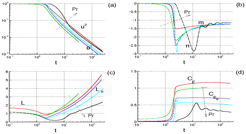
This work presents a comprehensive numerical validation of the Lyapunov-Liouville theoretical framework and its non-diffusive turbulence closures under freely decaying homogeneous isotropic turbulence (HIT). The closed system of von Karman-Howarth and Corrsin equations is integrated via an autonomous, high-accuracy architecture across three initial states (Saffman-Birkhoff, Loitsiansky, and Gaussian correlation profiles) and Prandtl numbers from Pr = 10^-3 to 1000. The analysis scrutinizes the transient phase, the self-preserving diffusive regime, and the internal structure of turbulence via velocity and temperature increment probability density functions (PDFs). Our findings reveal that the closure accurately captures distinct decay paths. The Saffman-Birkhoff case yields asymptotic exponents m = -1.25 and n = -1.25. The Loitsiansky condition accelerates mechanical decay (m = -1.51) due to higher dissipation but exhibits higher thermal persistence (n = -0.89). Conversely, the Gaussian profile induces ultra-rapid decay (m = -2.7), reaching its operational limit at t = 33 as R_lambda drops below 10. Furthermore, the model replicates the non-equilibrium evolution of characteristic scales. At Pr = 1000, the thermal microscale drops below the Kolmogorov scale, confirming Batchelor's scaling where the Batchelor constant converges to C_B = 3.5 and the Obukhov-Corrsin constant matches C_OC = 1.8. Finally, the synthesized PDFs capture a sharp transition from quasi-Gaussian statistics at low Pr to enhanced, scale-dependent small-scale intermittency at high Pr, validating the predictive robustness of the theory for multi-scale scalar mixing.
Figures




Reference graph
Works this paper leans on
-
[1]
Kolmogorov, A. N. (1941). The local structure of turbulence in incompressible viscous fluid for very large Reynolds numbers. Dokl. Akad. Nauk SSSR , Vol. 30, No. 4, pp. 299–303, 1941
1941
-
[2]
Obukhov, A. M. (1941). On the Energy Distribution in the Spectrum of a Turbulent Flow Dokl. Akad. Nauk SSSR , Vol. 32. , pp. 22–24, 1941. 58
1941
-
[3]
von K ´arm´an, T., & Howarth, L. (1938). On the statistical theory of isotropic turbulence. Proc. R. Soc. Lond. A , 164, 192-215
1938
-
[4]
Corrsin, S. (1951). On the spectrum of isotropic temperature fluc- tuations in an isotropic turbulence. Journal of Applied Physics , 22(4), 469-473
1951
-
[5]
, The Decay of Isotropic Temperature Fluctuations in an Isotropic Turbulence, Journal of Aeronautical Science, 18, pp
Corrsin S. , The Decay of Isotropic Temperature Fluctuations in an Isotropic Turbulence, Journal of Aeronautical Science, 18, pp. 417–423, no. 12, (1951)
1951
-
[6]
Millionshtchikov M. D. (1941). On the theory of homogeneous isotropic turbulence. Doklady Akademii Nauk SSSR , 32(9), 615–618
1941
-
[7]
, Zur Deutung der dreifachen Geschwindigkeitskorre- lationen der isotropen Turbulenz, Dtsch
Hasselmann K. , Zur Deutung der dreifachen Geschwindigkeitskorre- lationen der isotropen Turbulenz, Dtsch. Hydrogr. Z, 11, 5, 207-217, (1958)
1958
-
[8]
, Isotropic turbulence in the field of turbulent viscosity, JETP Lett., 8, 406–411, (1969)
Millionshtchikov M. , Isotropic turbulence in the field of turbulent viscosity, JETP Lett., 8, 406–411, (1969)
1969
-
[9]
, Closure of the two-point correlation equa- tion as a basis for Reynolds stress models, Appl
Oberlack M., Peters N. , Closure of the two-point correlation equa- tion as a basis for Reynolds stress models, Appl. Sci. Res. , 51, 533–539, (1993)
1993
-
[10]
Baev M. K. & Chernykh G. G. , On Corrsin equation closure, Journal of Engineering Thermophysics , 19, pp. 154–169, no. 3, (2010), DOI: 10.1134/S1810232810030069 59
-
[11]
A., Mellor G
Domaradzki J. A., Mellor G. L. , A simple turbulence closure hypothesis for the triple-velocity correlation functions in homogen eous isotropic turbulence, Jour. of Fluid Mech. , 140, 45–61, (1984)
1984
-
[12]
Orszag S. A. (1970). Analytical theories of turbulence. Journal of Fluid Mechanics , 41(2), 363–386, 1970,
1970
-
[13]
and Memari, S
Briard, A., Gomez, T., Sagaut, P. and Memari, S. (2016). Passive scalar decay laws in isotropic turbulence: Prandtl number e f- fects Journal of Fluid Mechanics , 787, 274–303
2016
-
[14]
Ottino J. M. (1989). The Kinematics of Mixing: Stretching, Chaos, and Transport. Cambridge Texts in Applied Mathematics, Cambridge University Press. ,
1989
-
[15]
de Divitiis, N. , Lyapunov Analysis for Fully Developed Homogeneous Isotropic Turbulence, Theoretical and Computational Fluid Dynamics , (2011), DOI: 10.1007/s00162-010-0211-9
-
[16]
de Divitiis, N. , Finite Scale Lyapunov Analysis of Temperature Fluc- tuations in Homogeneous Isotropic Turbulence, Appl. Math. Modell. , (2014), DOI: 10.1016/j.apm.2014.04.016
-
[17]
de Divitiis N. , von K´ arm´ an–Howarth and Corrsin equations clo- sure based on Lagrangian description of the fluid motion, An- nals of Physics , vol. 368, May 2016, Pages 296-309, (2016), DOI: 10.1016/j.aop.2016.02.010
-
[18]
de Divitiis, N. , Liouville spectral gap and bifurcation–driven Lagrangian-–Eulerian decoupling with nondiffusive turbulence clo- 60 sures Transport Phenomena 1, no. 1, 2026, pp. 20260015. https://doi.org/10.1515/tp-2026-0015
-
[19]
de Divitiis, N. , From bifurcations to state-variable statistics in isotropic turbulence: internal structure, intermittency, and Ko l- mogorov scaling via non-observable quasi-PDFs Transport Phenomena 1, no. 1, 2026, pp. 20260032. https://doi.org/10.1515/tp-2026- 0032
-
[20]
de Divitiis, N. , Quantitative evaluation of forward and backward scattering in isotropic turbulence via H¨ anggi–Klimontovich and Itˆ o stochastic processes Transport Phenomena 1, no. 2, 2026, pp. 20260054. https://doi.org/10.1515/tp-2026-0054
-
[21]
P., Chen, S., Brasseur, J
W ang, L. P., Chen, S., Brasseur, J. G., & Wyngaard, J. C. (1996). Examination of hypotheses in the Kolmogorov 1941 theory of turbulence of high-resolution direct numerical simulations. Journal of Fluid Mechanics , 309, 113-156
1996
-
[22]
and Uno, A
Kaneda, Y., Ishihara, T., Yokokawa, M., Itakura, K. and Uno, A. (2003). Energy dissipation rate and energy spectrum in high resolution direct numerical simulations of turbulence in a periodic box . Physics of Fluids , 15, no. 2, pp. L21–L24
2003
-
[23]
Comte-Bellot, G., & Corrsin, S. (1966). The use of a contracted transition section from a square to a linear cascade of grids for gen erat- ing isotropic turbulence. Journal of Fluid Mechanics , 25(4), 657-682
1966
-
[24]
Sreenivasan, Katepalli R. (1996). The passive scalar spectrum and the Obukhov–Corrsin constant. Physics of Fluids , 8(1), 189-196. 61
1996
-
[25]
W arhaft, Z. (2000). Passive scalars in turbulent flows. Annual Re- view of Fluid Mechanics , 32, 203-240
2000
-
[26]
, On sta- tistical correlations between velocity increments and locally averag ed dissipation in homogeneous turbulence, Phys
Chen S., Doolen G.D., Kraichnan R.H., She Z-S. , On sta- tistical correlations between velocity increments and locally averag ed dissipation in homogeneous turbulence, Phys. Fluids A , 5, pp. 458–463, (1992)
1992
-
[27]
, Numerical simulation of three- dimensional homogeneous isotropic turbulence., Phys
Orszag S.A., Patterson G.S. , Numerical simulation of three- dimensional homogeneous isotropic turbulence., Phys. Rev. Lett. , 28, 76–79, (1972)
1972
-
[28]
Orszag S.A., Yakhot V
Panda R., Sonnad V., Clementi E. Orszag S.A., Yakhot V. , Turbulence in a randomly stirred fluid, Phys. Fluids A , 1(6), 1045– 1053, (1989)
1989
-
[29]
, Effects of the similarity model in finite-difference LES of isotropic turbulence using a lagrangian dyna mic mixed model, Flow Turbul
Anderson R., Meneveau C. , Effects of the similarity model in finite-difference LES of isotropic turbulence using a lagrangian dyna mic mixed model, Flow Turbul. Combust. , 62, pp. 201–225, (1999)
1999
-
[30]
, On the representation of backscat- ter in dynamic localization models, Phys
Carati D., Ghosal S., Moin P. , On the representation of backscat- ter in dynamic localization models, Phys. Fluids , 7(3), pp. 606–616, (1995)
1995
-
[31]
, Decaying turbulence in an active–gridgenerated flow and comparisons with large–eddy simu la- tion., J
Kang H.S., Chester S., Meneveau C. , Decaying turbulence in an active–gridgenerated flow and comparisons with large–eddy simu la- tion., J. Fluid Mech. 480, pp. 129–160, (2003)
2003
-
[32]
Batchelor, G. K. , Small-scale variation of convected quantities like temperature in turbulent fluid. Part 1. General discussion and the case 62 of small conductivity, Journal of Fluid Mechanics , 5, (1959), pp. 113– 133
1959
-
[33]
K., Howells I
Batchelor G. K., Howells I. D., Townsend A. A. , Small-scale variation of convected quantities like temperature in turbulent fluid . Part 2. The case of large conductivity, Journal of Fluid Mechanics , 5, (1959), pp. 134–139
1959
-
[34]
Obukhov, A. M. , The structure of the temperature field in a turbu- lent flow. Dokl. Akad. Nauk. , CCCP, 39, (1949), pp. 391
1949
-
[35]
H., Schwarz W
Gibson, C. H., Schwarz W. H. , The Universal Equilibrium Spectra of Turbulent Velocity and Scalar Fields, Journal of Fluid Mechanics , 16, (1963), pp. 365–384
1963
-
[36]
, Passive scalar statistics in high- P´ eclet-number grid turbulence, Journal of Fluid Mechanics , 358, (1998), pp
Mydlarski, L., W arhaft, Z. , Passive scalar statistics in high- P´ eclet-number grid turbulence, Journal of Fluid Mechanics , 358, (1998), pp. 135–175
1998
-
[37]
Chasnov, J., Canuto V. M., Rogallo R. S. , Turbulence spec- trum of strongly conductive temperature field in a rapidly stirred flu id. Phys. Fluids A , 1, pp. 1698-1700, (1989), doi:10.1063/1.857535
doi:10.1063/1.857535 1989
-
[38]
Donzis D. A., Sreenivasan K. R., Yeung P. K. , The Batchelor Spectrum for Mixing of Passive Scalars in Isotropic Turbulence, Flow, Turbulence and Combustion , 85, pp. 549–566, no. 3–4, (2010), DOI: 10.1007/s10494-010-9271-6
-
[39]
, Introduction to nonlinear science , Cambridge University Press, (1995)
Nicolis, G. , Introduction to nonlinear science , Cambridge University Press, (1995). 63
1995
-
[40]
Taylor, G. I. (1935). Statistical theory of turbulence. Proceedings of the Royal Society of London. Series A , 151(873), 421-444
1935
-
[41]
Sreenivasan, K. R. (1984). On the scaling of the turbulence dissi- pation rate. Physics of Fluids , 27(5), 1048-1051
1984
-
[42]
V assilicos, J. C. (2015). Dissipation in turbulent flows. Annual Review of Fluid Mechanics , 47, 95-114
2015
-
[43]
Pope, S. B. (2000). Turbulent Flows. Cambridge University Press
2000
-
[44]
Rodhiya A., Sreenivasan, K. R. (2026). The Asymptotic State of Decaying Turbulence arXiv:2602.12501
Pith/arXiv arXiv 2026
-
[45]
Migdal A. (2026). Geometric Solution of Turbulence as Diffusion in Loop Space arXiv:2511.02165. 64
Pith/arXiv arXiv 2026
discussion (0)
Sign in with ORCID, Apple, or X to comment. Anyone can read and Pith papers without signing in.