REVIEW 4 major objections 6 minor 44 references
A Physics-Augmented GraphGPS Framework for the Reconstruction of 3D Riemann Problems from Sparse Data
T0 review · 4 major / 6 minor · reviewed 2026-08-07 · deepseek-v4-flash
Pith's one-line read This paper claims that a shock-aware graph-transformer recipe called GraphGPS can reconstruct 3D Riemann problem flow fields from only 10% of the data, with lower relative L2 error and sharper shocks than four standard machine-learning…
desk verdict A novel GraphGPS adaptation with real engineering value, but the 'superior accuracy' headline rests on single-run comparisons and test-set selection; merits peer review with demands for statistical rigor. read the letter →
The pith
A machine-rendered reading of the paper's core claim, the machinery that carries it, and where it could break.
The reading
What carries the argument
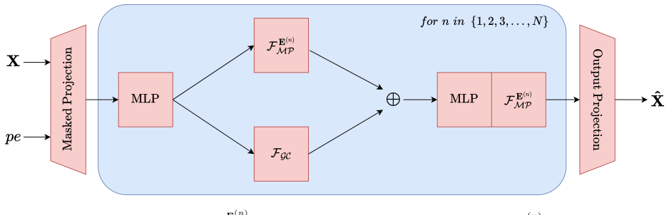
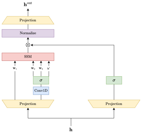
The load-bearing object is the GraphGPS layer stack, in which each layer splits into a local message-passing module and a global-context module, with residual connections and positional encodings. The paper's central modification is SA-GATConv, a graph-attention layer whose attention weights include extra learned terms applied to a physical-discontinuity feature tensor Z = (||∇ρ||2, ||∇p||2, max(0, -div(u,v,w))), stacked over time steps; this lets each node weight its neighbours more sharply where density or pressure jumps or where flow converges. The other machinery is guided message-passing, which constructs edge indices iteratively so that information flows only from nodes that were known initially or have already received information, and masked projection, which zeroes the learned representation of unknown nodes so the network sees only their positional encodings. Training uses two separate Adam optimizers: one for a data loss on known nodes and one for a Godunov loss that evaluates the reconstructed conserved fields through HLLC approximate Riemann fluxes.
What would settle it
Re-train the same architecture on ground truth produced by a different high-order solver, such as an exact Riemann solver or an ADER scheme, on the same six configurations, and compare relative L2 errors and shock sharpness against the four benchmarks; if SA-GATConv's edge shrinks or reverses, the reported superiority is tied to HLLC-WENO's numerical biases rather than to a general reconstruction ability.
Extended reading notes
Core claim
The paper's central claim is stated in Section 4.3: the GraphGPS model with SA-GATConv message-passing, Mamba-2 global context, guided message-passing, and masked projection has superior accuracy compared to all benchmarks for every one of the six 3D Riemann cases, while also producing sharper reconstructions of shocks, slip lines, and rarefaction fans. SA-GATConv is the key new message-passing layer: it augments the standard graph-attention score with learned terms acting on a feature tensor Z, assembled from per-node density-gradient magnitude, pressure-gradient magnitude, and negative velocity divergence, so the aggregation weights become aware of discontinuities. The paper further claims that guided message-passing matches dense message-passing in accuracy while reducing time and memory and improving early training stability, and that masked projection makes reconstruction agnostic to the initialization of unknown nodes without hurting accuracy. The ablation study supports the claim that, for this task, the local message-passing choice matters more than the global-context module.
Load-bearing premise
The benchmark that everything is measured against is one particular numerical solver's output, and the physics loss is built from one approximate flux formula; if the model has learned the quirks of that solver rather than the actual flow physics, the accuracy gains may not survive contact with other solvers or real sensors.
Editorial extensions
If this is right
- If correct, the same recipe should reconstruct other shock-dominated 3D flows from sparse sensor data, such as transonic or supersonic aerodynamics, with less smearing at discontinuities.
- Guided message-passing makes graph-based reconstruction sparser, cheaper, and more stable without sacrificing accuracy, which matters for scaling to finer grids and larger domains.
- Masked projection removes the need for feature propagation or other initialization heuristics for unknown nodes, simplifying the training pipeline.
- The ablation result that local message-passing matters more than global context suggests future effort should focus on improving local aggregation rather than global attention modules.
- Because the framework beats GAT, linear transformer, autoencoder, and 3D CNN baselines, it provides a stronger baseline for future sparse-flow reconstruction work.
Reading between the lines
- The reported superiority is measured against ground truth from HLLC-WENO; a natural extension is to test whether the model transfers to fields generated by other high-order schemes or to experimental data, which would reveal whether it learns genuine physics or the numerical solver's artifacts.
- The per-case training setup suggests a harder, untested claim: one model trained on several Riemann configurations and sensor masks might generalize across configurations; the architecture's modularity makes this plausible but the paper does not demonstrate it.
- Since Z uses only density and pressure gradients plus velocity divergence, the same shock-awareness trick could be applied to other hyperbolic systems, such as magnetohydrodynamics or shallow-water flows, where analogous jump conditions exist.
- The memory overhead of attention-based message-passing is the stated bottleneck; replacing the attention score computation with a cheaper linear or kernelized form that preserves shock awareness is a concrete path to finer resolutions.
Editorial analysis
A structured set of objections, weighed in public.
Referee Report
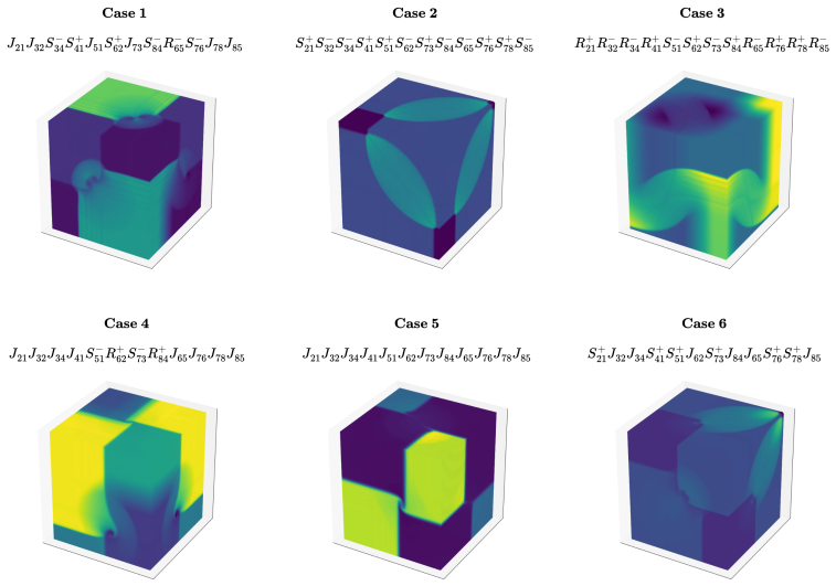
Summary. The paper proposes a GraphGPS-based deep learning architecture for reconstructing 3D Riemann problem fields (density, velocity components, and pressure) from sparse measurements with 90% of nodes unknown. The main contributions are: (i) SA-GATConv, a shock-aware graph attention layer that incorporates physical gradients from the previous epoch's reconstruction into the attention weights; (ii) guided message-passing, which restricts information flow to originate from known nodes and expands the known set over layers; (iii) masked projection that zeroes unknown-node representations in the latent space to make reconstruction agnostic to the initialization of unknown values; and (iv) an application of the GraphGPS framework to a new SciML problem. The model is trained with a data loss on known nodes plus a physics-based Godunov loss using HLLC flux residuals. The authors report ablations over message-passing layers, global-context modules, connectivity parameter λ, and projection type, and benchmark their selected architecture against GAT, linear transformer, autoencoder, and 3D CNN on six 3D Riemann cases, claiming superior accuracy in all cases.
Significance. If the results are statistically robust, this is a useful application-driven contribution to scientific ML for compressible flows. The work is, to the best of the authors' claim, the first to use GraphGPS for flow-field reconstruction and the first SciML study of 3D Riemann problems. The modular ablation of message-passing and global-context components is valuable, and the release of code and data supports reproducibility. The shock-aware attention mechanism and guided message-passing are reasonable architectural novelties. However, the central claim of superior accuracy is not yet statistically grounded: all reported errors come from single training runs with a single random mask, with no error bars, repeated seeds, or paired significance tests, and the architecture is selected on the same six cases used for the headline benchmark comparison. In addition, the contribution of the physics-informed loss is never isolated in an ablation, leaving the 'physics-augmented' element unquantified.
major comments (4)
- [Section 4.3, Fig. 12, Table 4, Eq. (6)] The central claim that the proposed model has 'superior accuracy compared to the benchmarks for all cases' rests entirely on single training runs per model/case and a single random mask drawn from Eq. (6). No error bars, confidence intervals, or repeated seeds are reported anywhere in the paper. This matters because the ablation of Section 4.1 states that SA-GATConv is only 'slightly lower' in error than plain GATConv, so the margins shown in Fig. 12 could be within run-to-run variability. The authors should repeat each experiment with multiple random masks and initialization seeds (at least 3–5, ideally more), and report the mean and standard deviation of the relative L2 error for each model and case, together with a paired significance test (e.g., a paired t-test or Wilcoxon signed-rank test) across the six cases. Without this, the claimed superiority is not statistically established.
- [Section 4.1 vs Section 4.3] The ablation study selects the final architecture (SA-GATConv for F_MP, Mamba-2 for F_GC, λ=3, masked projection) by comparing errors on the same six Riemann cases that are then used in Section 4.3 to benchmark against GAT, transformer, autoencoder, and 3D CNN. There is no independent validation set or cross-validation procedure. This means the headline benchmark comparison is partially a selection-on-the-test-set result: the chosen configuration is the one that performed best on the very cases used for the final evaluation, which inflates the reported advantage and undermines the unbiasedness of the comparison. The authors should either reserve one or more cases (or distinct mask draws) for model selection and use them for validation, or report the performance of all ablated variants in the Section 4.3 comparison so that the reader can see whether the selected configuration is an outlier. An explicit statement of what constitutes the validation split is essential.
- [Section 3.4 and Section 4] The paper's title and abstract emphasize a 'physics-augmented' model, and Section 3.4 introduces a physics loss L_phy based on HLLC flux residuals. However, no experiment compares training with L_data only against training with L_data + L_phy. As a result, the contribution of the physics-informed loss to reconstruction accuracy or shock sharpness is never measured. This is load-bearing for the central claim that the proposed 'physics-augmented' approach is beneficial. The authors should add an ablation that trains the same architecture with and without L_phy under identical settings and reports the relative L2 errors and visual quality for all six cases. This would also inform the interpretation of the HLLC-WENO coupling: if the physics loss is essential, the choice of HLLC as the flux estimator and its relation to the WENO-generated training data becomes a more delicate question; if it is not essential, the 'physics-augmented' label should be adjusted accordingly.
- [Section 3.1, Eq. (5)] The positivity-preserving transformation T is stated to be applied 'during training' after F_Θ, but the manuscript does not explicitly state whether T is also part of the forward pass at inference time. If T is omitted during evaluation, the model may output negative density or pressure, contradicting the claim of a hard positivity constraint. If T is always applied as part of the model's forward pass, this should be stated explicitly in Section 3.1 or 3.3. The authors should clarify this point and, if T is intended only as a training-time transformation, justify why it guarantees positive outputs at deployment.
minor comments (6)
- [Appendix A, Eq. (A.2)] The second wave speed in Eq. (A.2) is labeled 's l' but appears to be a typo; it should be 's_r = u_tilde + a_tilde', matching the left speed s_l = u_tilde - a_tilde.
- [Appendix B, Eq. (B.1)] The sign of the last term in the expression for α0 appears to be incorrect for the standard 5th-order WENO reconstruction; the standard form uses +11/6 U_i, while the manuscript writes -11/6 U_i.
- [Section 3.3 (first paragraph)] The sentence 'The number of layers N is determined by the size of the set of edge indices' is unclear. The size of a set is not a number of layers; please rephrase and explicitly state how N is chosen and what value of N is used in the experiments.
- [Section 4 (experimental setup)] The temporal setup of the reconstruction task is not fully specified: the number of timesteps N_t, the final simulation time, and the meaning of 'time resolution 5×10^-4' are missing. Without this information, the reader cannot fully interpret the input/output feature dimension N_tc = N_t * N_c or the physics loss in Eq. (26).
- [Section 4.2] The feature-propagation baseline used for the unmasked projection comparison is mentioned without a formal description or algorithmic definition; please provide a brief explanation or a specific citation to a concrete feature-propagation method.
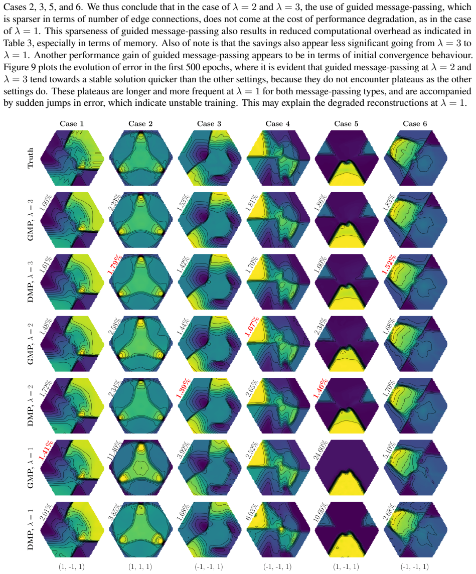
- [Figures 6–12] The relative L2 error values printed in the subplots are small and sometimes difficult to read; consider enlarging the font size or also reporting the numerical values in a table, especially for the repeated-run results that should be added per the major comments.
Circularity Check
No significant circularity: the reconstruction pipeline is self-contained, with only a minor non-load-bearing self-citation to the authors' Godunov-loss paper.
full rationale
The derivation chain is self-contained. The sparse data are defined by the random mask in Eq. (6); the data loss Ldata in Eq. (25) supervises only the known nodes; the physics loss Lphy in Eqs. (26)-(29) penalizes HLLC flux residuals of the model output; and the reported error metric in Eq. (7) is a separate relative L2 norm against the HLLC-WENO ground truth. None of these quantities is defined in terms of another in a way that would force the reconstructed accuracy. In particular, Lphy is not a function of the ground-truth field, and the model must still interpolate 90% missing points, so the use of the same HLLC solver family in the loss and in the target generator is an inductive bias rather than a circular reduction. The only self-citation is [41], used to justify the Godunov loss; the loss itself is fully specified in this paper, and the headline benchmark claim in Section 4.3 rests on empirical comparisons (Fig. 12) against external GAT, transformer, autoencoder, and 3D CNN baselines, so the self-citation is not load-bearing. The selection of SA-GATConv, Mamba-2, lambda=3, and masked projection on the same six cases used for the headline comparison is a statistical limitation (no held-out validation set, no repeated seeds or error bars), but it is model selection on the test set rather than a constructional equivalence, and therefore does not constitute circularity.
Assumptions & free parameters
free parameters (5)
- lambda (neighborhood connectivity) =
3
- hidden channels =
64
- learning rate =
1e-4
- number of global attention heads =
16
- sparsity mask fraction =
0.9 unknown
assumptions (5)
- domain assumption 3D Euler equations with Neumann boundary conditions govern the flow.
- domain assumption HLLC approximate Riemann solver provides accurate inter-cell fluxes.
- domain assumption 5th-order WENO reconstruction produces accurate ground-truth fields.
- domain assumption The GraphGPS framework [21] provides a suitable base architecture.
- domain assumption Literature Riemann initial conditions are valid canonical configurations.
Cite this review
Pith. "Pith review of A Physics-Augmented GraphGPS Framework for the Reconstruction of 3D Riemann Problems from Sparse Data." pith.science (2026). https://pith.science/paper/VDGR4IM4
@misc{pith2026250521421,
  author       = {Pith},
  title        = {Pith review of: A Physics-Augmented GraphGPS Framework for the Reconstruction of 3D Riemann Problems from Sparse Data},
  year         = {2026},
  howpublished = {\url{https://pith.science/paper/VDGR4IM4}},
  note         = {Machine review of arXiv:2505.21421}
}
read the original abstract
In compressible fluid flow, reconstructing shocks, discontinuities, rarefactions, and their interactions from sparse measurements is an important inverse problem with practical applications. Moreover, physics-informed machine learning has recently become an increasingly popular approach for performing reconstructions tasks. In this work we explore a machine learning recipe, known as GraphGPS, for reconstructing canonical compressible flows known as 3D Riemann problems from sparse observations, in a physics-informed manner. The GraphGPS framework combines the benefits of positional encodings, local message-passing of graphs, and global contextual awareness, and we explore the latter two components through an ablation study. Furthermore, we modify the aggregation step of message-passing such that it is aware of shocks and discontinuities, resulting in sharper reconstructions of these features. Additionally, we modify message-passing such that information flows strictly from known nodes only, which results in computational savings, better training convergence, and no degradation of reconstruction accuracy. We also show that the GraphGPS framework outperforms numerous machine learning benchmarks.
Figures

Figures from the paper (9 more)




Reference graph
Works this paper leans on
-
[1]
The graph neural network model,
F. Scarselli, M. Gori, A. C. Tsoi, M. Hagenbuchner, and G. Monfardini, “The graph neural network model,”IEEE transactions on neural networks, vol. 20, no. 1, pp. 61–80, 2008
2008
-
[2]
Semi-supervised classification with graph convolutional networks,
T. N. Kipf and M. Welling, “Semi-supervised classification with graph convolutional networks,”arXiv preprint arXiv:1609.02907, 2016
arXiv 2016
-
[3]
P. Veličković, G. Cucurull, A. Casanova, A. Romero, P. Lio, and Y. Bengio, “Graph attention networks,”arXiv preprint arXiv:1710.10903, 2017
arXiv 2017
-
[4]
Inductive representation learning on large graphs,
W. Hamilton, Z. Ying, and J. Leskovec, “Inductive representation learning on large graphs,”Advances in neural information processing systems, vol. 30, 2017
2017
-
[5]
How powerful are graph neural networks?
K. Xu, W. Hu, J. Leskovec, and S. Jegelka, “How powerful are graph neural networks?”arXiv preprint arXiv:1810.00826, 2018
arXiv 2018
-
[6]
Neural machine translation by jointly learning to align and translate,
D. Bahdanau, K. Cho, and Y. Bengio, “Neural machine translation by jointly learning to align and translate,”arXiv preprint arXiv:1409.0473, 2014
arXiv 2014
-
[7]
Effectiveapproachestoattention-basedneuralmachinetranslation,
M.-T.Luong,H.Pham,andC.Manning,“Effectiveapproachestoattention-basedneuralmachinetranslation,” arXivpreprintarXiv:1508.04025 , 2015
arXiv 2015
-
[8]
A. Vaswani, N. Shazeer, N. Parmar, J. Uszkoreit, L. Jones, A. Gomez, L. Kaiser, and I. Polosukhin, “Attention is all you need,”Advances in Neural Information Processing Systems, 2017
work page 2017
Show all 44 references
-
[9]
Improving language understanding by generative pre-training,
A. Radford, K. Narasimhan, T. Salimans, and I. Sutskever, “Improving language understanding by generative pre-training,” 2018
2018
-
[10]
Bert: Pre-training of deep bidirectional transformers for language understanding,
J. Devlin, M.-W. Chang, K. Lee, and K. Toutanova, “Bert: Pre-training of deep bidirectional transformers for language understanding,” in Proceedings of naacL-HLT, vol. 1, no. 2. Minneapolis, Minnesota, 2019
2019
-
[11]
An image is worth 16x16 words: Transformers for image recognition at scale,
A.Dosovitskiy,L.Beyer,A.Kolesnikov,D.Weissenborn,X.Zhai,T.Unterthiner,M.Dehghani,M.Minderer,G.Heigold,S.Gelly,J.Uszkoreit, and N. Houlsby, “An image is worth 16x16 words: Transformers for image recognition at scale,”arXiv preprint arXiv: 2010.11929, 2020
2010 arXiv
-
[12]
Transformers are rnns: Fast autoregressive transformers with linear attention,
A. Katharopoulos, A. Vyas, N. Pappas, and F. Fleuret, “Transformers are rnns: Fast autoregressive transformers with linear attention,” in International conference on machine learning. PMLR, 2020, pp. 5156–5165
2020
-
[13]
Rethinking attention with performers,
K. Choromanski, V. Likhosherstov, D. Dohan, X. Song, A. Gane, T. Sarlos, P. Hawkins, J. Davis, A. Mohiuddin, L. Kaiseret al., “Rethinking attention with performers,”arXiv preprint arXiv:2009.14794, 2020
2009 arXiv
-
[14]
Mamba: Linear-time sequence modeling with selective state spaces,
A. Gu and T. Dao, “Mamba: Linear-time sequence modeling with selective state spaces,”arXiv preprint arXiv:2312.00752, 2023
2023 arXiv
-
[15]
Transformers are ssms: Generalized models and efficient algorithms through structured state space duality,
T. Dao and A. Gu, “Transformers are ssms: Generalized models and efficient algorithms through structured state space duality,”arXiv preprint arXiv:2405.21060, 2024
2024 arXiv
-
[16]
A generalization of transformer networks to graphs,
V. P. Dwivedi and X. Bresson, “A generalization of transformer networks to graphs,”arXiv preprint arXiv:2012.09699, 2020
2012 arXiv
-
[17]
Rethinking graph transformers with spectral attention,
D. Kreuzer, D. Beaini, W. Hamilton, V. Létourneau, and P. Tossou, “Rethinking graph transformers with spectral attention,”Advances in Neural Information Processing Systems, vol. 34, pp. 21618–21629, 2021
2021
-
[18]
Do transformers really perform badly for graph representation?
C. Ying, T. Cai, S. Luo, S. Zheng, G. Ke, D. He, Y. Shen, and T.-Y. Liu, “Do transformers really perform badly for graph representation?” Advances in neural information processing systems, vol. 34, pp. 28877–28888, 2021
2021
-
[19]
Graph mamba: Towards learning on graphs with state space models,
A. Behrouz and F. Hashemi, “Graph mamba: Towards learning on graphs with state space models,” inProceedings of the 30th ACM SIGKDD conference on knowledge discovery and data mining, 2024, pp. 119–130
2024
-
[20]
Graph-mamba: Towards long-range graph sequence modeling with selective state spaces,
C. Wang, O. Tsepa, J. Ma, and B. Wang, “Graph-mamba: Towards long-range graph sequence modeling with selective state spaces,”arXiv preprint arXiv:2402.00789, 2024
2024 arXiv
-
[21]
Recipe for a general, powerful, scalable graph transformer,
L. Rampášek, M. Galkin, V. P. Dwivedi, A. T. Luu, G. Wolf, and D. Beaini, “Recipe for a general, powerful, scalable graph transformer,” Advances in Neural Information Processing Systems, vol. 35, pp. 14501–14515, 2022
2022
-
[22]
On the unreasonable effectiveness of feature propagation in learning on graphs with missing node features,
E. Rossi, H. Kenlay, M. I. Gorinova, B. P. Chamberlain, X. Dong, and M. M. Bronstein, “On the unreasonable effectiveness of feature propagation in learning on graphs with missing node features,” inProceedings of the First Learning on Graphs Conference. PMLR, 2022
2022
-
[23]
Karhunen–loeve procedure for gappy data,
R. Everson and L. Sirovich, “Karhunen–loeve procedure for gappy data,”JOSA A, vol. 12, no. 8, pp. 1657–1664, 1995
1995
-
[24]
Aerodynamic data reconstruction and inverse design using proper orthogonal decomposition,
T. Bui-Thanh, M. Damodaran, and K. Willcox, “Aerodynamic data reconstruction and inverse design using proper orthogonal decomposition,” AIAA journal, vol. 42, no. 8, pp. 1505–1516, 2004
2004
-
[25]
Proper orthogonal decomposition for steady aerodynamic applications,
A. Vendl and H. Faßbender, “Proper orthogonal decomposition for steady aerodynamic applications,”PAMM, vol. 10, no. 1, pp. 635–636, 2010
2010
-
[26]
A surrogate-based flow-field prediction and optimization strategy for hypersonic thrust nozzle,
H. Huang, Q. Wang, and Z. Wu, “A surrogate-based flow-field prediction and optimization strategy for hypersonic thrust nozzle,”AIP Advances, vol. 14, no. 12, 2024
2024
-
[27]
Graph neural networks for aerodynamic flow reconstruction from sparse sensing,
G. Duthé, I. Abdallah, S. Barber, and E. Chatzi, “Graph neural networks for aerodynamic flow reconstruction from sparse sensing,”arXiv preprint arXiv:2301.03228, 2023
2023 arXiv
-
[28]
A practical approach to flow field reconstruction with sparse or incomplete data through physics informed neural network,
S. Xu, Z. Sun, R. Huang, D. Guo, G. Yang, and S. Ju, “A practical approach to flow field reconstruction with sparse or incomplete data through physics informed neural network,”Acta Mechanica Sinica, vol. 39, no. 3, p. 322302, 2023
2023
-
[29]
Gappy ae: A nonlinear approach for gappy data reconstruction using auto-encoder,
Y. Kim, Y. Choi, and B. Yoo, “Gappy ae: A nonlinear approach for gappy data reconstruction using auto-encoder,”Computer Methods in Applied Mechanics and Engineering, vol. 426, p. 116978, 2024
2024
-
[30]
Rapid and sparse reconstruction of high-speed steady-state and transient compressible flow fields using physics-informed graph neural networks,
J.-Z. Peng, Z.-Q. Wang, X. Rong, M. Mei, M. Wang, Y. He, and W.-T. Wu, “Rapid and sparse reconstruction of high-speed steady-state and transient compressible flow fields using physics-informed graph neural networks,”Physics of Fluids, vol. 36, no. 4, 2024
2024
-
[31]
Flow field reconstruction from sparse sensor measurements with physics-informed neural networks,
M. Y. Hosseini and Y. Shiri, “Flow field reconstruction from sparse sensor measurements with physics-informed neural networks,”Physics of Fluids, vol. 36, no. 7, 2024
2024
-
[32]
Flow reconstruction in time-varying geometries using graph neural networks,
B. A. Danciu, V. A. Pagone, B. Böhm, M. Schmidt, and C. E. Frouzakis, “Flow reconstruction in time-varying geometries using graph neural networks,”arXiv preprint arXiv:2411.08764, 2024
2024 arXiv
-
[33]
Graph neural networks and differential equations: A hybrid approach for data assimilation of fluid flows,
M. Quattromini, M. A. Bucci, S. Cherubini, and O. Semeraro, “Graph neural networks and differential equations: A hybrid approach for data assimilation of fluid flows,”arXiv preprint arXiv:2411.09476, 2024
2024 arXiv
-
[34]
Flrnet: A deep learning method for regressive reconstruction of flow field from limited sensor measurements,
P. C. Nguyen, J. B. Choi, and Q.-T. Luu, “Flrnet: A deep learning method for regressive reconstruction of flow field from limited sensor measurements,”arXiv preprint arXiv:2411.13815, 2024
2024 arXiv
-
[35]
Flronet: Deep operator learning for high-fidelity fluid flow field reconstruction from sparse sensor measurements,
H. V. Dang, J. B. Choi, and P. C. Nguyen, “Flronet: Deep operator learning for high-fidelity fluid flow field reconstruction from sparse sensor measurements,”arXiv preprint arXiv:2412.08009, 2024. 19
2024
-
[36]
On the choice of wavespeeds for the HLLC riemann solver,
P. Batten, N. Clarke, C. Lambert, and D. M. Causon, “On the choice of wavespeeds for the HLLC riemann solver,”SIAM Journal on Scientific Computing, vol. 18, no. 6, pp. 1553–1570, 1997
1997
-
[37]
Classification of the Riemann problem for two-dimensional gas dynamics,
C. W. Schulz-Rinne, “Classification of the Riemann problem for two-dimensional gas dynamics,”SIAM journal on mathematical analysis, vol. 24, no. 1, pp. 76–88, 1993
1993
-
[38]
Asystematicanalysisofthree-dimensionalriemannproblemsforverification of compressible-flow solvers,
N.Hoppe,N.Fleischmann,B.Biller,S.Adami,andN.A.Adams,“Asystematicanalysisofthree-dimensionalriemannproblemsforverification of compressible-flow solvers,”Computers & Fluids, vol. 278, p. 106298, 2024
2024
-
[39]
Benchmarking graph neural networks,
V. P. Dwivedi, C. K. Joshi, A. T. Luu, T. Laurent, Y. Bengio, and X. Bresson, “Benchmarking graph neural networks,”Journal of Machine Learning Research, vol. 24, no. 43, pp. 1–48, 2023
2023
-
[40]
Exphormer: Sparse transformers for graphs,
H. Shirzad, A. Velingker, B. Venkatachalam, D. J. Sutherland, and A. K. Sinop, “Exphormer: Sparse transformers for graphs,” inInternational Conference on Machine Learning. PMLR, 2023, pp. 31613–31632
2023
-
[41]
Godunov loss functions for modelling of hyperbolic conservation laws,
R. Cassia and R. Kerswell, “Godunov loss functions for modelling of hyperbolic conservation laws,”Computer Methods in Applied Mechanics and Engineering, vol. 437, p. 117782, 2025
2025
-
[42]
The HLLC Riemann solver,
E. F. Toro, “The HLLC Riemann solver,”Shock Waves, vol. 29, no. 8, pp. 1065–1082, 2019
2019
-
[43]
Springer Science & Business Media, 2013
——, Riemann solvers and numerical methods for fluid dynamics: a practical introduction. Springer Science & Business Media, 2013
2013
-
[44]
Threedimensionalhllriemannsolverforconservationlawsonstructuredmeshes;applicationtoeulerandmagnetohydrodynamic flows,
D.S.Balsara,“Threedimensionalhllriemannsolverforconservationlawsonstructuredmeshes;applicationtoeulerandmagnetohydrodynamic flows,”Journal of Computational Physics, vol. 295, pp. 1–23, 2015. 20 Appendix A. HLLC Flux Estimation Figure A.1: The three-wave model assumed by the HL...
2015
Reviewed August 7, 2026 · model on record in the stance chip above.
Discussion (0). Sign in to comment.