REVIEW 4 major objections 5 minor 40 references
Extreme Event Aware ($\eta$-) Learning
T0 review · 4 major / 5 minor · reviewed 2026-08-04 · deepseek-v4-flash
Pith's one-line read η-learning enforces a prescribed observable law during training, so a surrogate can generate unprecedented extremes even when the training data contain no extreme examples.
desk verdict A coherent regularized-ERM framework for enforcing prescribed extreme statistics, but the headline 'no extreme data needed' claim rests on an externally supplied reference measure that the experiments mostly take from ground truth. read the letter →
The pith
A machine-rendered reading of the paper's core claim, the machinery that carries it, and where it could break.
The reading
What carries the argument
The central object is the push-forward distribution ϕ#µ of a candidate map through the one-dimensional observable g, compared to a reference law ν0 by the 1-Wasserstein distance. In one dimension W1 has the quantile formula ∫ |F^{-1}_{ϕ#µ}(q) − F^{-1}_{ν0}(q)| dq, so the regularizer is evaluated on an upper-tail set of quantiles (τ around 0.95–0.99) rather than globally. Two supporting mechanisms carry the argument: the data-consistent estimator definition and Theorem 4 lower bound (supervised estimators leave an unavoidable tail gap), and the Inference-Informed Continual Training algorithm, which identifies the few quantile-triggering inputs and observable-active dimensions so that W1 backp
What would settle it
On a system with known ground truth, construct a training set whose inputs deliberately avoid the extreme set, set ν0 to the true y#µ, and compute W1 between yη#µ and y#µ on a large held-out sample. If the tail gap is statistically indistinguishable from the MSE estimator's tail gap, or if the η-map's output distribution tracks ν0 only in the bulk, the central claim fails. A sharper version: use a deliberately misspecified ν0 (for example, the wrong heavy-tail exponent) and check whether yη#µ follows the wrong law; this would show the method cannot create correct extremes without accurate refe
Extended reading notes
Core claim
The central claim is that absence of extreme data can be compensated by statistical information about an extreme-relevant observable. Formally, for a data-consistent estimator yξ (one that fits well outside the extreme set E but errs more inside it), when n ≤ log p / log(1−δ), the W1 distance between true and estimated push-forward measures obeys W1(y#µ, yξ#µ) ≥ (1−C̃)|∫_E (y−yξ) dµ|, so ordinary supervised learning cannot vanish tail error in the data-scarce regime. Adding W1(ϕ#µ, ν0) to the ERM objective yields yη; under stated assumptions this regularizer is optimal in the sense that W1(yη#µ, y#µ) is equivalent, up to constants, to the extreme-region L1 error ∫_E |yη−y| dµ. With ν0 = y#µ,
Load-bearing premise
The reference distribution ν0 is known, accurate, and available before training; if the extreme tail is itself unknown, the method can only match whatever distribution it is handed, and the paper offers no procedure to certify ν0 from data that lack extremes.
Editorial extensions
If this is right
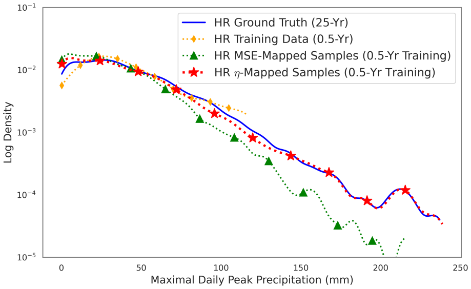
- A downscaler trained on 0.5 years of high-resolution data, with no extremes in that slice, can produce daily precipitation fields whose spatial-maximum distribution matches the 25-year reference tail beyond quantile 150.
- η-learning acts as a model-agnostic statistical corrector: pushing samples from a low-resolution generative model through the η-map lifts their observable tails to match the high-resolution reference.
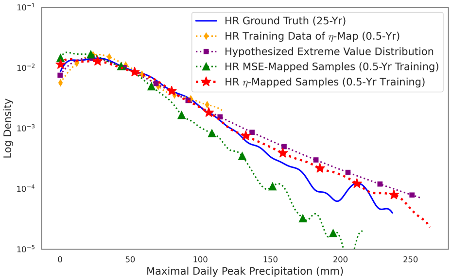
- With a hypothesized heavier-tailed generalized extreme value distribution as ν0, the map generates extreme precipitation fields more severe than any observed, enabling what-if extremes for climate risk assessment.
- The optimality theorems imply W1 is not an arbitrary choice: under the stated assumptions, minimizing W1 specifically minimizes the expected absolute error in the extreme set.
- The η-learned candidates are not unique but can guide active data acquisition or quantify epistemic uncertainty in extreme regions.
Reading between the lines
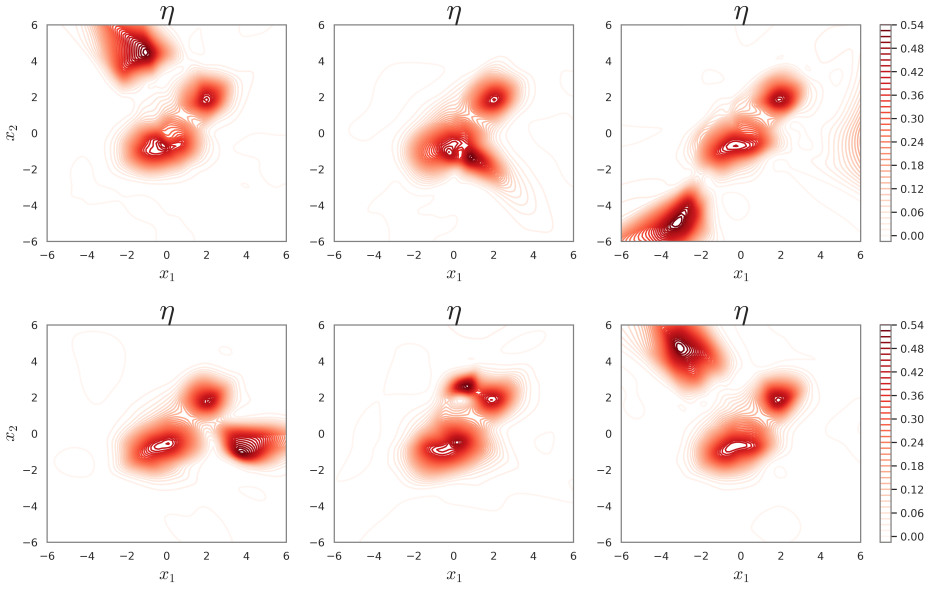
- The method is distribution-only: it matches the observable law, not the spatial location of extremes. For risk mapping that needs to know where an extreme occurs, a spatial prior or downstream localization would be required; the paper's own middle-column example shows η can create an extreme where the truth has none.
- The practical bottleneck left open is certification of ν0 from data that lack extremes; all but one experiment use the true y#µ. A data-driven procedure that audits a candidate ν0 without extreme samples would turn the method from a proof-of-concept into a deployable tool.
- The same mechanism should transfer to other sparse-event domains such as financial shocks, rogue waves, or grid failures whenever a physically or statistically motivated tail law exists; the observable g only needs to be a one-dimensional severe-event indicator.
- Because W1 in one dimension has an analytic quantile form and the regularization is applied only on upper quantiles, the method is a natural add-on to any supervised or generative model rather than a bespoke architecture.
Editorial analysis
A structured set of objections, weighed in public.
Referee Report
Summary. The paper introduces η-learning, a supervised-learning framework augmented by a 1-Wasserstein regularization term that enforces prescribed output statistics (a reference measure ν0) for an observable indicative of extremeness. The central claim is that, even when training data contain no extreme events, matching the observable's push-forward distribution to ν0 reduces epistemic uncertainty in extreme regions and enables generation of unprecedented extremes. The theory introduces 'data-consistent estimators' and proves lower bounds on W1(y#µ, yξ#µ) and related optimality results, all formulated under the ideal assumption ν0 = y#µ. Five experiments are presented: two toy problems and three precipitation downscaling applications, with the final application using a hypothesized heavy-tailed GEVD as ν0. The method is practical via a quantile-based W1 approximation and an inference-informed continual training algorithm.
Significance. If the central claim were fully established, η-learning would be a valuable contribution: it offers a principled way to inject statistical prior knowledge about extremes into surrogate models and provides a concrete algorithmic framework (quantile-based W1 regularization, IICT) for doing so. The theoretical development around data-consistent estimators is a useful attempt to formalize why ERM fails in extreme regions. The precipitation downscaling experiments, especially the generative-model correction and the hypothesized-tail experiment, demonstrate a plausible use case. The paper also shows robustness of the method to the balancing hyperparameter λ. However, the load-bearing part of the claim — that absence of extreme data can be compensated by statistical information — is empirically supported only in a circular way in four of five experiments, because ν0 is set to the ground-truth push-forward. The final GEVD experiment shows matching a prescribed heavy tail, not recovering an unknown true tail. The theoretical results are conditional on unverified constants and assumptions. With additional non-ideal ν0 experiments and clearer positioning of the theoretical conditions, the con
major comments (4)
- [§7, 'General experiment protocols'; Figs. 4, 7, 11] Four of the five experiments set ν0 = y#µ (the exact ground-truth push-forward, constructed from 10^6 evaluations or the full 25-year dataset as described in App. F.1/F.3). Since the training objective in Eqs. (11)-(12) directly minimizes W1(φ#µ, ν0), the observed tail agreement in Figs. 4, 7, and 11 is enforced by construction rather than discovered. These experiments therefore validate that the optimizer can minimize the regularizer, but they do not provide independent evidence for the paper's central claim that a surrogate trained without extreme examples can produce output statistics matching a prescribed extreme law ν0 when ν0 is not already the ground truth. The one non-ideal experiment (§7.5) uses a GEVD fitted to the same 25-year ground-truth observables and then manually made heavier; it demonstrates consistency with a prescribed hypothesis, not recovery of an unknown tail. I re
- [§3, Definition 3, Eqs. (6)-(9)] The data-consistent estimator definition assumes the existence of constants C~, C^ < 1 satisfying inequalities (6)-(9). The paper explicitly states that these constants are 'challenging, if infeasible, to verify precisely' and that the <1 property is only 'hypothesize[d]'. Yet Theorem 4 (Eq. (10)), Theorem 6, and Theorem 7 all rely on these constants. As written, the results are conditional on an unverified structural condition rather than a proven property of ERM or neural-network estimators. The paper's motivational claim that 'commonly employed supervised-learning estimators fail' is therefore not established for any concrete function class used in the experiments. Please either (a) prove or numerically demonstrate that typical NN classes satisfy Definition 3 with C~, C^ < 1 on the test problems, or (b) explicitly state these as assumptions and temper the 'fundamental limitation' clai
- [§5, Theorem 9; App. C, proof of Theorem 17] Theorem 9 only establishes that, as K→1 and under Assumptions 8a/8b, W1(yη#µ, y#µ) is within ε1+ε2 of ∫_E |yη−y|dµ. This does not prove that minimizing W1 minimizes the extreme-region L1 error; the additive errors ε1, ε2 depend on yξ and are not shown to be small or controllable in the actual optimization. Moreover, the practical objective in Eq. (21) replaces W1 by a tail-truncated quantile sum over [τ,1] with τ chosen manually (0.95–0.989), so the theory's assumptions (full W1, ν0=y#µ, K→1) are not satisfied in the experiments. The optimality claims in Section 5 are therefore substantially weaker than stated. Please revise to state the precise conditions under which the equivalence holds and clarify the gap between the theoretical objective and the implemented one.
- [§7.5, App. F.5] The final experiment uses a hypothesized GEVD that is fitted to the ground-truth observables and then manually made heavier (σ increased by 4). The resulting yη#µ matches this hypothesized distribution, producing events more extreme than any observed. This is a valid demonstration that the method can enforce a prescribed tail hypothesis, but it does not provide evidence that the method can identify the correct extreme law from data that lack extremes. The paper's abstract claims that statistics can be 'obtained from qualitative knowledge or unlabeled data'; this experiment does not exercise that pathway. I recommend adding either an unlabeled-data-based ν0 experiment or a misspecification study showing how the output tail deviates when ν0 is wrong, so readers can assess the robustness of the method to the central input.
minor comments (5)
- [Abstract] The phrase 'e2a or eta' appears to be an incomplete formatting artifact; the symbol is later introduced as η-learning. Please clean up.
- [§3, Eqs. (7),(9)] The notations C~ and C^ are defined through an 'inf C≥0' that is unusual because the infimum of the set {C≥0 : inequality} is often 0 if the numerator is zero; the authors likely mean the smallest constant such that the inequality holds. Please clarify the definition to avoid ambiguity.
- [Fig. 2 caption] The caption says '2D-to-1D toy example' but the section describes a 2D-to-2D problem. Please correct.
- [Fig. 17 caption] Two curves are both labeled '0.5-year data' (the dotted olive with circles and the dotted dark green with flipped triangles). One likely refers to the 2.5-year or another training amount; please fix the labels.
- [App. E, Eq. (20)] The quantile estimator uses g(φ(x~(⌈n_x q_i⌉))) but the text says 'j-th largest value'; please ensure the order statistic notation is consistent with the sorting direction used in Algorithm 2.
Circularity Check
Central validation and optimality claims reduce to the training objective under the ideal assumption ν0 = y#µ; the 'no-extreme-data' result is not independently demonstrated.
-
fitted input called prediction
[Section 7 'General experiment protocols', with Eqs. (11)-(12) and Appendices F.1/F.3]
"Specifically, we consistently operate under the ideal assumption that ν0 = y#µ attaching to our developed theory—except in the final application, where ν0 is indeed hypothesized. The process of obtaining a certified ν0, if not available a priori, is application-specific and thus beyond the scope of this work."
Eq. (11) defines yη as the minimizer of ERM loss plus λ·W1(φ#µ, ν0). In four of the five experiments ν0 is taken to be the ground-truth push-forward y#µ, constructed in the toy examples from 1,000,000 exact evaluations of y and in the precipitation example from the full 25-year HR dataset. Therefore the regularizer is literally W1(φ#µ, y#µ), and the reported agreement yη#µ ≈ y#µ (Figs. 4, 7, 11) is the minimization target itself, not a prediction about unknown extremes. The claim that η-learning 'enables the generation of unprecedented extreme events' is conditioned on the extreme statistics already being present in ν0; the experiments validate that the optimizer minimizes its own loss rather than that a certified ν0 can be obtained from data lacking extremes.
-
self definitional
[Section 5, paragraph after Theorem 9]
"recall that yη is defined to minimize W1(yη#µ, y#µ). Given this equivalence, minimizing W1(yη#µ, y#µ) inherently leads to the minimization of R E |yη −y|dµ."
Under the 'ideal assumption that ν0 = y#µ' stated at the start of Section 5, the optimality theorem reduces to analyzing the quantity that yη is defined to minimize. The conclusion that W1(yη#µ, y#µ) controls the extreme-region L1 error is a property of the chosen objective when the reference equals the ground truth; it does not establish that a reference obtainable without extreme data would have this property. Thus the theoretical 'optimality' arguments inherit the same conditioning on ν0 = y#µ and do not by themselves support the no-extreme-data headline claim.
full rationale
The paper's internal derivation is coherent in parts: Theorem 4's lower bound for data-consistent estimators and the W1 upper/lower bound lemmas are proved from explicit assumptions and are not themselves circular. The circularity enters at the load-bearing junction between the method, the theory, and the experiments. Eq. (11) defines η-learning as minimizing ERM plus λ·W1(φ#µ, ν0). The experiments and the optimality section then set ν0 = y#µ, with ν0 obtained from 10^6 exact evaluations of the true map or from the full 25-year high-resolution dataset. With that choice, matching y#µ is the training objective, so the observed tail agreement in Figs. 4, 7, and 11 is a check that the regularizer was minimized, not an external validation that extreme statistics can be recovered without extreme information. Theorem 9's statement that minimizing W1(yη#µ, y#µ) minimizes the extreme-region error is likewise a property of the chosen objective under the ideal assumption. The single non-ideal experiment (§7.5) demonstrates only that the method matches a prescribed heavier GEVD, which is again the objective by construction; it does not certify that hypothesized distribution. The paper explicitly defers 'obtaining a certified ν0' to future work, so the central premise—that the relevant extreme statistics are known a priori—is assumed rather than derived or independently tested. This is a partial but central circularity: the headline capability is validated by feeding the ground-truth output distribution into the term that the method is designed to minimize. Score 7 rather than higher because the framework itself, the data-consistency lower bound, and the conditional statement 'if ν0 is correct, the output tail matches ν0' are internally consistent and have independent content.
Assumptions & free parameters
free parameters (4)
- λ (W1 regularization weight) =
1.0 in most experiments; 1e-4...10 in robustness test
- τ (tail cutoff for quantile matching) =
0.989 (downscaling), 0.95 (GEVD experiment)
- Quantile grid Q =
explicit lists in App F.1, F.2, F.3, F.5
- GEVD reference parameters =
κ=-0.179, ζ=25.077, σ=21.928→25.928, γ=0.00470
assumptions (6)
- ad hoc to paper There exist constants C~, C^<1 such that any data-consistent estimator's non-extreme error is bounded by its extreme error (Def. 3 (6)-(9))
- ad hoc to paper Assumption 5: ∫_E |yξ-y| dμ ≤ K |∫_E (yξ-y) dμ| for K≥1
- domain assumption Assumptions 8a/8b: non-extreme errors of yξ and yξ-yη are small (ε1, ε2)
- domain assumption Input distribution µ is known and cheaply sampleable (or has abundant samples)
- domain assumption A faithful reference measure ν0 is available before training
- domain assumption The theory for y transfers to the state map u through g
Cite this review
Pith. "Pith review of Extreme Event Aware ($\eta$-) Learning." pith.science (2026). https://pith.science/paper/VF2HG2IB
@misc{pith2026251019161,
  author       = {Pith},
  title        = {Pith review of: Extreme Event Aware ($\eta$-) Learning},
  year         = {2026},
  howpublished = {\url{https://pith.science/paper/VF2HG2IB}},
  note         = {Machine review of arXiv:2510.19161}
}
abstract
Quantifying and predicting rare and extreme events is challenging because such events are infrequent, severe, and expensive to simulate. Existing data-driven methods often require multiple extremes in the training data or sampling process, leading to accurate predictions in quiescent regimes but high epistemic uncertainty in extreme-event regions. To overcome this limitation, we introduce Extreme Event Aware ($\eta$-) Learning, which does not require extreme events in the available data. The method reduces uncertainty even in uncharted extreme regimes by enforcing during training the statistics of an observable indicative of extremeness, obtained from qualitative knowledge or unlabeled data. This statistical regularization results in models that fit observed data while remaining consistent with prescribed observable statistics, enabling the generation of unprecedented extreme events. Optimal-transport-based theoretical results offer rigorous justification and establish key optimality properties. Numerical experiments on prototype systems and real-world precipitation downscaling problems demonstrate the effectiveness of the $\eta$-learning framework.
Figures


Figures from the paper (15 more)




Reference graph
Works this paper leans on
-
[1]
MIT press, 2024
Francis Bach.Learning theory from first principles. MIT press, 2024
2024
-
[2]
Benedikt Barthel Sorensen, Alexis Charalampopoulos, Shixuan Zhang, BE Harrop, LR Leung, and Themistoklis P Sapsis. A non-intrusive machine learning framework for debiasing long-time coarse resolution climate simulations and quantifying rare events statistics.Journal of Advances in Modeling Earth Systems, 16(3):e2023MS004122, 2024
2024
-
[3]
Distribution tail structure and extreme value analysis of constrained piecewise linear oscillators
Vadim Belenky, Dylan Glotzer, Vladas Pipiras, and Themistoklis P Sapsis. Distribution tail structure and extreme value analysis of constrained piecewise linear oscillators. Probabilistic Engineering Mechanics, 57:1–13, 2019
2019
-
[4]
Bayesian optimization with output- weighted optimal sampling.Journal of Computational Physics, 425:109901, 2021
Antoine Blanchard and Themistoklis Sapsis. Bayesian optimization with output- weighted optimal sampling.Journal of Computational Physics, 425:109901, 2021
2021
-
[5]
Sinho Chewi, Jonathan Niles-Weed, and Philippe Rigollet. Statistical optimal transport. arXiv preprint arXiv:2407.18163, 2024
arXiv 2024
-
[6]
Springer, 2001
Stuart Coles, Joanna Bawa, Lesley Trenner, and Pat Dorazio.An introduction to sta- tistical modeling of extreme values, volume 208. Springer, 2001
2001
-
[7]
Cousins and T
W. Cousins and T. P. Sapsis. Reduced order precursors of rare events in unidirectional nonlinear water waves.Journal of Fluid Mechanics, 790:368–388, 2016
2016
-
[8]
Sinkhorn distances: Lightspeed computation of optimal transport.Ad- vances in neural information processing systems, 26, 2013
Marco Cuturi. Sinkhorn distances: Lightspeed computation of optimal transport.Ad- vances in neural information processing systems, 26, 2013
2013
Show all 40 references
-
[9]
Rogue waves and large deviations in deep sea.Proceedings of the National Academy of Sciences, 115(5):855– 860, 2018
Giovanni Dematteis, Tobias Grafke, and Eric Vanden-Eijnden. Rogue waves and large deviations in deep sea.Proceedings of the National Academy of Sciences, 115(5):855– 860, 2018
2018
-
[10]
Asymptotic theory for the probability density functions in burgers turbulence.Physical Review Letters, 83(13):2572–2575, 1999
Weinan E and Eric Vanden-Eijnden. Asymptotic theory for the probability density functions in burgers turbulence.Physical Review Letters, 83(13):2572–2575, 1999
1999
-
[11]
Transition-path theory and path-finding algorithms for the study of rare events.Annual review of physical chemistry, 61:391–420, jan 2010
Weinan E and Eric Vanden-Eijnden. Transition-path theory and path-finding algorithms for the study of rare events.Annual review of physical chemistry, 61:391–420, jan 2010
2010
-
[12]
John Wiley & Sons, 1999
Gerald B Folland.Real analysis: modern techniques and their applications, volume 40. John Wiley & Sons, 1999
1999
-
[13]
Cambridge University Press, 2011
Jean-Pierre Fouque, George Papanicolaou, Ronnie Sircar, and Knut Sølna.Multiscale stochastic volatility for equity, interest rate, and credit derivatives. Cambridge University Press, 2011
2011
-
[14]
On choosing and bounding probability metrics
Alison L Gibbs and Francis Edward Su. On choosing and bounding probability metrics. International statistical review, 70(3):419–435, 2002
2002
-
[15]
MIT press, 2016
Ian Goodfellow, Yoshua Bengio, and Aaron Courville.Deep learning. MIT press, 2016. 24
2016
-
[16]
Adam: A method for stochastic optimization.arXiv preprint arXiv:1412.6980, 2014
Diederik P Kingma. Adam: A method for stochastic optimization.arXiv preprint arXiv:1412.6980, 2014
2014 arXiv
-
[17]
A Tutorial on Energy-Based Learning
Yann Lecun, Sumit Chopra, and Raia Hadsell. A Tutorial on Energy-Based Learning. InPredicting Structured Data, number January 2016. MIT Press, 2006
2016
-
[18]
Flow matching for generative modeling.arXiv preprint arXiv:2210.02747, 2022
Yaron Lipman, Ricky TQ Chen, Heli Ben-Hamu, Maximilian Nickel, and Matt Le. Flow matching for generative modeling.arXiv preprint arXiv:2210.02747, 2022
2022 arXiv
-
[19]
A one-dimensional model for dispersive wave turbulence.Journal of Nonlinear Science, 7:9–44, 1997
Andrew J Majda, David W McLaughlin, and EG1431687 Tabak. A one-dimensional model for dispersive wave turbulence.Journal of Nonlinear Science, 7:9–44, 1997
1997
-
[20]
Sequential sampling strategy for extreme event statistics in nonlinear dynamical systems.Proceedings of the National Academy of Sciences, 115(44):11138–11143, 2018
Mustafa A Mohamad and Themistoklis P Sapsis. Sequential sampling strategy for extreme event statistics in nonlinear dynamical systems.Proceedings of the National Academy of Sciences, 115(44):11138–11143, 2018
2018
-
[21]
Era5-land: A state-of-the-art global reanalysis dataset for land applications.Earth system science data, 13(9):4349–4383, 2021
Joaqu ´ ın Mu˜ noz-Sabater, Emanuel Dutra, Anna Agust ´ ı-Panareda, Cl´ ement Albergel, Gabriele Arduini, Gianpaolo Balsamo, Souhail Boussetta, Margarita Choulga, Shaun Harrigan, Hans Hersbach, et al. Era5-land: A state-of-the-art global reanalysis dataset for land application...
2021
-
[22]
Univariate stable distributions.Springer Series in Operations Research and Financial Engineering, 10:978–3, 2020
John P Nolan. Univariate stable distributions.Springer Series in Operations Research and Financial Engineering, 10:978–3, 2020
2020
-
[23]
Pytorch: An imperative style, high-performance deep learning library.Advances in neural infor- mation processing systems, 32, 2019
Adam Paszke, Sam Gross, Francisco Massa, Adam Lerer, James Bradbury, Gregory Chanan, Trevor Killeen, Zeming Lin, Natalia Gimelshein, Luca Antiga, et al. Pytorch: An imperative style, high-performance deep learning library.Advances in neural infor- mation processing systems, 32, 2019
2019
-
[24]
Discovering and forecasting extreme events via active learning in neural operators.Na- ture Computational Science, 2(12):823–833, 2022
Ethan Pickering, Stephen Guth, George Em Karniadakis, and Themistoklis P Sapsis. Discovering and forecasting extreme events via active learning in neural operators.Na- ture Computational Science, 2(12):823–833, 2022
2022
-
[25]
U-net: Convolutional networks for biomedical image segmentation
Olaf Ronneberger, Philipp Fischer, and Thomas Brox. U-net: Convolutional networks for biomedical image segmentation. InMedical image computing and computer-assisted intervention–MICCAI 2015: 18th international conference, Munich, Germany, October 5-9, 2015, proceedings, part I...
2015
-
[26]
The Wasserstein distances between pushed-forward measures with ap- plications to uncertainty quantification.Communications in Mathematical Sciences, 18(3):707–724, June 2020
Amir Sagiv. The Wasserstein distances between pushed-forward measures with ap- plications to uncertainty quantification.Communications in Mathematical Sciences, 18(3):707–724, June 2020. Publisher: International Press of Boston
2020
-
[27]
Statistics of extreme events in fluid flows and waves.Annual Review of Fluid Mechanics, 53(1):85–111, 2021
Themistoklis P Sapsis. Statistics of extreme events in fluid flows and waves.Annual Review of Fluid Mechanics, 53(1):85–111, 2021
2021
-
[28]
Themistoklis P Sapsis and Antoine Blanchard. Optimal criteria and their asymptotic form for data selection in data-driven reduced-order modelling with gaussian process regression.Philosophical Transactions of the Royal Society A, 380(2229):20210197, 2022. 25
2022
-
[29]
Weather and climate extreme events in a changing climate.Climate Change 2021: The Physical Science Basis
Sonia I Seneviratne, Xuebin Zhang, Muhammad Adnan, Wafae Badi, Claudine Dereczynski, A Di Luca, Subimal Ghosh, Iskhaq Iskandar, James Kossin, Sophie Lewis, et al. Weather and climate extreme events in a changing climate.Climate Change 2021: The Physical Science Basis. Contribu...
2021
-
[30]
Sobczyk.Stochastic Differential Equations
K. Sobczyk.Stochastic Differential Equations. Kluwer Academic Publishers, Dordrecht, The Netherlands, 1991
1991
-
[31]
Soong and M
T. Soong and M. Grigoriu.Random Vibration of Mechanical and Structural Systems. PTR Prentice Hall, 1993
1993
-
[32]
A probabilistic framework for learn- ing non-intrusive corrections to long-time climate simulations from short-time training data.arXiv preprint arXiv:2408.02688, 2024
Benedikt Barthel Sorensen, Leonardo Zepeda-N´ u˜ nez, Ignacio Lopez-Gomez, Zhong Yi Wan, Rob Carver, Fei Sha, and Themistoklis Sapsis. A probabilistic framework for learn- ing non-intrusive corrections to long-time climate simulations from short-time training data.arXiv prepri...
2024 arXiv
-
[33]
Sullivan, M
T. Sullivan, M. Koslowski, F. Theil, and M. Ortiz. On the behavior of dissipative systems in contact with a heat bath: Application to Andrade creep.Journal of the Mechanics and Physics of Solids, 57(7):1058–1077, 2009
2009
-
[34]
M. A. Tayfun. Narrow-band nonlinear sea waves.Journal of Geophysical Research, 85(C3):1548, 1980
1980
-
[35]
Large deviation theory-based adaptive importance sampling for rare events in high dimensions.SIAM/ASA Journal on Uncertainty Quan- tification, 11(3):788–813, 2023
Shanyin Tong and Georg Stadler. Large deviation theory-based adaptive importance sampling for rare events in high dimensions.SIAM/ASA Journal on Uncertainty Quan- tification, 11(3):788–813, 2023
2023
-
[36]
Oliphant, Matt Haberland, Tyler Reddy, David Cournapeau, Evgeni Burovski, Pearu Peterson, Warren Weckesser, Jonathan Bright, St´ efan J
Pauli Virtanen, Ralf Gommers, Travis E. Oliphant, Matt Haberland, Tyler Reddy, David Cournapeau, Evgeni Burovski, Pearu Peterson, Warren Weckesser, Jonathan Bright, St´ efan J. van der Walt, Matthew Brett, Joshua Wilson, K. Jarrod Millman, Nikolay Mayorov, Andrew R. J. Nelson,...
2020
-
[37]
Practicalities and Algorithmic Details
Yinhao Zhu, Nicholas Zabaras, Phaedon Stelios Koutsourelakis, and Paris Perdikaris. Physics-constrained deep learning for high-dimensional surrogate modeling and uncer- tainty quantification without labeled data.Journal of Computational Physics, 394:56– 81, 2019. 26 A Missing ...
2019
-
[38]
Importantly, all other hyperparameters (e.g., learning rate, number of epochs) were held fixed in this experiment, further confirming robustness with respect toλ. F.2 The 2D-to-2D Toy Problem In this example, we model the intermediate state mapuas follows: u(x1, x2) = u1(x1, x...
1999
-
[39]
The window sizeωin Algorithm 1 is selected to be 30, and we train the network for 150 epochs
with a learning rate of 0.0003. The window sizeωin Algorithm 1 is selected to be 30, and we train the network for 150 epochs. Additionally, another neural network is trained under identical configurations to compute an MSE estimator for baseline comparison. After training, we ...
-
[40]
The testing and evaluation procedures stay the same as the vanilla case. 45 Figure 8: The contour plot of 6 more independent realizations of theη-estimator trained with the same dataset and reference distribution as the realization shown in the rightmost plot of Fig. 1. 46 Fig...
Reviewed August 4, 2026 · model on record in the stance chip above.
Discussion (0). Continue with ORCID to comment.