REVIEW 3 major objections 5 minor 56 references
Sparse Sensor Allocation for Inverse Problems of Detecting Sparse Leaking Emission Sources
T0 review · 3 major / 5 minor · reviewed 2026-08-15 · deepseek-v4-flash
Pith's one-line read The central claim: sensor placement for sparse leak detection can be solved as a bilevel optimization whose outer objective is the wind-averaged mean squared estimation error of a nonnegative elastic-net inverse solver.
desk verdict A promising sensor-placement framework with a real gap in the hypergradient derivation: the SBA update likely descends a partial derivative that ignores how sampled data depend on sensor locations. read the letter →
The pith
A machine-rendered reading of the paper's core claim, the machinery that carries it, and where it could break.
The reading
What carries the argument
The load-bearing object is the bilevel formulation (11) with the nonnegative elastic-net inverse problem (12) as its lower level and the wind-averaged IMSE as its upper objective. Its mechanism is the implicit-differentiation formula (17)-(18) for the hypergradient: differentiate the KKT conditions of the lower-level QP with respect to sensor locations, keeping only the active constraints (positions pinned at zero), to obtain the gradient that drives sensor updates. Around this sits an augmented primal-dual algorithm for solving each inner QP and a stochastic-approximation outer loop that re-samples wind and emission scenarios each step.
What would settle it
In a small case with a degenerate lower-level solution (a true zero coefficient whose optimal Lagrange multiplier is also zero), compute the hypergradient from (17)-(18) and compare it with a central finite-difference gradient of the IMSE; a mismatch beyond numerical tolerance would show the descent direction is not the true gradient.
Extended reading notes
Core claim
The paper's central claim is that the sensor layout itself should be chosen as the solution of the bilevel program (11): minimize the Monte Carlo estimate of $\mathbb{E}_{\theta,\beta,\Phi}\lVert \hat\theta(\Phi,\beta,s)-\theta\rVert_2^2$, where each $\hat\theta$ is the solution of a convex quadratic program imposing $\theta\ge 0$ with elastic-net penalties. Because the lower-level solver is differentiable through its KKT conditions under strict complementarity, the paper obtains the gradient of the upper-level objective with respect to sensor positions and uses it in two algorithms: rSAA, which repeats small sample-average problems and averages their outputs, and SBA, a stochastic projected-gradient method that re-samples wind and emissions each iteration. The convergence analysis shows the SBA iterate reaches a stationary point as the inner solver accuracy and batch size grow, and the numerical experiments report that in the 10-sensor/20-source test the mean absolute percentage error drops from 69.06% (random), to 50.79% (A-optimal start), to 29.94% (bilevel-optimized design).
Load-bearing premise
The hypergradient formula that drives every SBA sensor update assumes strict complementarity in the lower-level QP: every source whose estimated rate is pinned at zero must have a strictly positive dual multiplier, which can fail for elastic-net penalties when zero sits inside the L1 subdifferential.
Editorial extensions
If this is right
- Sensor layouts become functions of the wind distribution: with prevailing north-to-south wind, the algorithm places sensors along the downwind boundary, and reversing the wind rose would mirror the layout.
- The same machinery carries physical constraints other than nonnegativity (e.g., bounds, couplings) as long as the lower-level estimator remains a differentiable QP.
- Because the design objective is the estimation error of the actual sparse estimator rather than a posterior covariance proxy, the method can be applied whenever the inverse solver is regularized.
- The MAPE reduction reported in the 10-sensor/20-source validation brings the optimized design near the ~30% uncertainty ceiling used in methane quantification guidelines with fewer sensors than naive designs.
- The rSAA stochastic upper bound gives operators a computable certificate on how far a candidate placement is from the true optimum.
Reading between the lines
- A testable extension is to replace the strict-complementarity assumption with an epsilon-active-set or proximal differentiation rule; if the current hypergradient is biased on degenerate elastic-net solutions, such a fix would restore the descent property without changing the bilevel structure.
- The formulation should extend to other uncertain forward parameters (source height, diffusivity, atmospheric stability) by adding them to the sampling distribution, since the IMSE averaging does not depend on the parameter being wind.
- Because the paper's final layout is sensitive to initialization in nonconvex experiments, a practical deployment rule would be to run SBA from several starting designs (A-optimal, support points, random) and select by the rSAA-style confidence bound.
- For nonlinear dispersion models, the same bilevel objective could be paired with a learned differentiable surrogate of the inverse map, which is the paper's stated future direction.
Signed reviews
Editorial analysis
A structured set of objections, weighed in public.
Referee Report
Summary. The paper considers the sparse placement of sensors for estimating sparse, nonnegative emission sources under uncertain wind conditions. It formulates the problem as a bilevel optimization: the upper level minimizes the wind-averaged integrated mean squared error (IMSE) of the emission-rate estimates over sensor locations, while the lower level solves a nonnegative elastic-net-regularized inverse problem for each Monte Carlo scenario. Two algorithms are proposed: a repeated sample average approximation (rSAA) using a global solver on small deterministic problems, and a stochastic gradient-based bilevel approximation (SBA) that differentiates through the lower-level KKT system. Convergence bounds are stated for both methods, and numerical experiments with Gaussian-plume synthetic data compare the resulting designs against random, A-optimal, support-point, and other initial designs. Open-source GPU-accelerated code is provided.
Significance. If the central derivation were correct, the paper would offer a practical, scalable design tool that extends classical A-optimal experimental design to non-Gaussian, sparsity-promoting, physically constrained inverse problems with uncertain forward-model parameters. The formulation is a natural and useful extension, the numerical study covers a range of problem sizes, and the availability of reproducible code with GPU support is a concrete strength. However, the paper's main algorithmic claim for SBA is undercut by an apparently missing term in the hypergradient derivation, and the convergence guarantee rests on an unverified strict-complementarity assumption. The framework itself remains viable and the identified flaw is local and correctable, so the contribution is potentially significant but not yet established as stated.
major comments (3)
- [Section 3.2, Eq. (18) and Appendix A.1] The implicit differentiation of the KKT conditions treats the observations Phi^(i) as independent of s, but in Eqs. (5)-(7) the data are generated as Phi^(i)(s) = F(beta^(i),s) theta^(i) + epsilon^(i), so nabla_s Phi^(i) = (nabla_s F) theta^(i) is generally nonzero. The derivative of d^(i)(s) = lambda_2 1 - sigma_epsilon^{-2} F^*(beta^(i),s) Phi^(i)(s) therefore contains the additional term -sigma_epsilon^{-2} F^*(beta^(i),s) (nabla_s F(beta^(i),s)) theta^(i), which is absent from (18). Appendix B derives only derivatives of the plume kernel A_j(s_i), not the derivative of Phi with respect to s. Consequently, the SBA update (19) is not an unbiased stochastic gradient of the objective in (11a)/(6) unless this term is included, and Theorem 1's convergence statement applies to a different functional. This issue is load-bearing for the claim that SBA minimizes the IMSE; the rSAA algorithm may be unaffected, but the paper does not specify whether its sample generation re-evaluates Phi at each candidate sensor location s.
- [Section 3.2, paragraph after Proposition 2] The hypergradient formula requires strict complementarity, namely positive dual multipliers bar{eta} > 0 on all active constraints, but the paper neither proves this for the nonnegative elastic-net QP (12) nor verifies it numerically. For L1-type regularized problems, an active coordinate can have a zero dual multiplier when the subgradient at zero contains zero, in which case the active set is not differentiable and the implicit-function argument behind (18) breaks down. Since Lemma 1 and Theorem 1 are built on this differentiation, the convergence guarantee is conditional on an unverified assumption. The authors should either prove that strict complementarity holds generically for the Gaussian-plume forward model with lambda_1, lambda_2 > 0, or report numerical checks (e.g., the minimum of bar{eta} over active constraints across all iterations and Monte Carlo samples).
- [Section 4.4, Figure 19] The headline MAPE values (69.06%, 50.79%, and 29.94% for random, A-optimal initial, and proposed designs) are reported as single point estimates without standard errors, confidence intervals, or multiple independent replications. Because the objective (6) is stochastic in theta, beta, and Phi, and because Figure 12 shows that SBA converges to different local optima from different initializations, the Section 5 claim that the proposed approach 'can significantly improve the accuracy of the inverse estimation over some of the existing designs' is not fully substantiated. The authors should report means and dispersions over at least several independent runs, and state whether the same random seeds or Monte Carlo samples were used across the compared designs.
minor comments (5)
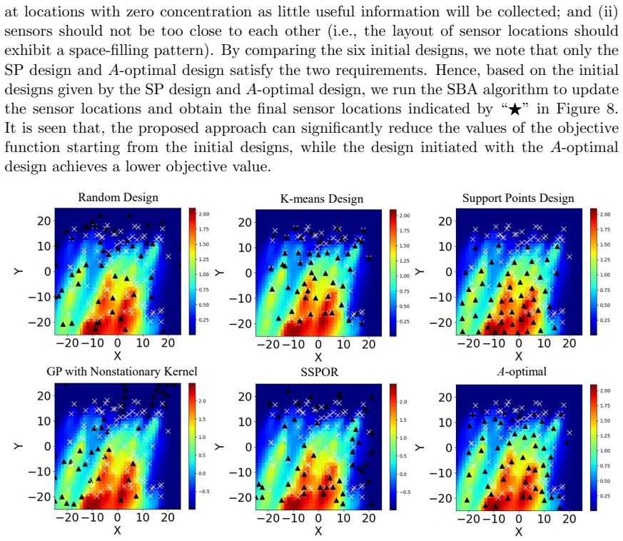
- [Abstract and Section 4.2] The abstract says the approach reduces IMSE 'starting from various initial sensor deployment generated by existing approaches,' but in Example II only the Support Points and A-optimal designs are actually used to initialize SBA; the random, K-means, GP, and SSPOR designs appear only in the qualitative comparison of Figure 7. The final validation in Section 4.4 uses random, A-optimal, and the proposed design. The wording should be made consistent with the experiments.
- [Appendix C.2] The proof of Theorem 1 invokes 'Assumption 7,' but only Assumptions 1-6 are stated anywhere in the paper. In the proof of Lemma 1 in Appendix C.1, the bound labeled 'according to Assumption 6' appears to require Assumption 5, the Lipschitz condition on D(s,hat{theta}(xi),hat{eta}(xi)). The assumptions should be renumbered and cross-referenced consistently.
- [Algorithm 1 and Section 3.3] The paper refers to 'existing global solvers' for the deterministic bilevel problems in rSAA but does not name the solver, the reformulation used, or the software. Since the reproducibility of the rSAA results depends on this, a concrete reference or implementation detail would be helpful.
- [Notation throughout] The symbol hat{Psi} is used both for the Monte Carlo sample-average objective (7) and for the true IMSE (6); in Theorem 1 and its proof, expressions such as hat{Psi}(s_m; theta*) and Psi(s_0; theta*) mix the two without definition. Please disambiguate these, for example by writing Psi for the true objective and hat{Psi}_N for the sample average.
- [Section 4.3] The sentence 'the iteration number M is chosen according to the computing budget' gives no criterion or sensitivity analysis for M. Since Figures 10-16 show trajectories and final designs for varying M, a brief statement on convergence monitoring or stopping rules would improve reproducibility.
Circularity Check
No circularity: the bilevel objective and the lower-level estimator are independently defined, and the numerical validation is benchmarked against external designs.
full rationale
The paper's derivation chain is self-contained and does not reduce to its own inputs. The upper-level objective (6) is an independent Monte Carlo expectation of the squared estimation error over stated priors for wind, emission rates, and observation noise, while the lower-level estimator (11b) is defined by an elastic-net-regularized, nonnegativity-constrained quadratic program. The sensor-allocation problem is not defined in terms of its own solution: the estimator is fixed first, and the sensor locations are then chosen to minimize the resulting IMSE. The hypergradient in Proposition 2 is obtained by implicit differentiation of the lower-level KKT conditions (Appendix A.1), and the convergence analysis in Theorem 1 is a standard stochastic-gradient argument rather than a restatement of the objective. The numerical validation re-evaluates the IMSE with large independent Monte Carlo samples and compares against external initial designs including random, K-means, Support Points, GP, SSPOR, and A-optimal placements, so the claimed improvement is an empirical benchmark result rather than a construction. Self-citations to Liu et al. (2022) for the global solver and to Liu and Yeo (2023) and Yeo et al. (2019) for the absence of closed-form solutions are supporting references for standard facts or implementation tools, and they do not carry the central derivation. A possible omission of the derivative of the sampled data with respect to sensor locations in the hypergradient expression (18) would be a correctness issue, not a circularity issue, because it does not make the output equivalent to the input by definition.
Assumptions & free parameters
free parameters (2)
- lambda1 (ridge penalty) =
0.0001, 0.01, 0.001 in examples
- lambda2 (lasso penalty) =
0.0001, 0.01, 0.001 in examples
assumptions (7)
- domain assumption Strict complementarity for the lower-level QP active set
- standard math Lipschitz smoothness of hypergradient (Assumption 1)
- domain assumption Lower-level optimality gap bounded by delta (Assumption 2)
- standard math Bounded gradient constants (Assumptions 3 to 6)
- domain assumption Gaussian plume forward model
- domain assumption Known prior distributions p(theta) and p(beta)
- domain assumption Background emission rate set to zero
Cite this review
Pith. "Pith review of Sparse Sensor Allocation for Inverse Problems of Detecting Sparse Leaking Emission Sources." pith.science (2026). https://pith.science/paper/VJPHYYRU
@misc{pith2026250905559,
  author       = {Pith},
  title        = {Pith review of: Sparse Sensor Allocation for Inverse Problems of Detecting Sparse Leaking Emission Sources},
  year         = {2026},
  howpublished = {\url{https://pith.science/paper/VJPHYYRU}},
  note         = {Machine review of arXiv:2509.05559}
}
read the original abstract
This paper investigates the sparse optimal allocation of sensors for detecting sparse leaking emission sources. Because of the non-negativity of emission rates, uncertainty associated with parameters in the forward model, and sparsity of leaking emission sources, the classical linear Gaussian Bayesian inversion setup is limited and no closed-form solutions are available. By incorporating the non-negativity constraints on emission rates, relaxing the Gaussian distributional assumption, and considering the parameter uncertainties associated with the forward model, this paper provides comprehensive investigations, technical details, in-depth discussions and implementation of the optimal sensor allocation problem leveraging a bilevel optimization framework. The upper-level problem determines the optimal sensor locations by minimizing the Integrated Mean Squared Error (IMSE) of the estimated emission rates over uncertain wind conditions, while the lower-level problem solves an inverse problem that estimates the emission rates. Two algorithms, including the repeated Sample Average Approximation (rSAA) and the Stochastic Gradient Descent based bilevel approximation (SBA), are thoroughly investigated. It is shown that the proposed approach can further reduce the IMSE of the estimated emission rates starting from various initial sensor deployment generated by existing approaches. Convergence analysis is performed to obtain the performance guarantee, and numerical investigations show that the proposed approach can allocate sensors according to the parameters and output of the forward model. Computationally efficient code with GPU acceleration is available on GitHub so that the approach readily applicable.
Figures


Figures from the paper (24 more)






Reference graph
Works this paper leans on
- [1]
-
[2]
Antil, H., Z. W. Di, and R. Khatri (2020). Bilevel optimization, deep learning and fractional laplacian regularization with applications in tomography. Inverse Problems\/ 36\/ (6), 064001
work page 2020
-
[3]
Attia, A., S. Leyffer, and T. Munson (2023). Robust a-optimal experimental design for bayesian inverse problems. arXiv preprint arXiv:2305.03855v1\/
arXiv 2023
-
[4]
Brunton, B. W., S. L. Brunton, J. L. Proctor, and J. N. Kutz (2016). Sparse sensor placement optimization for classification. SIAM Journal on Applied Mathematics\/ 76\/ (5), 2099--2122
work page 2016
-
[5]
Chen, Q., M. Modi, G. McGaughey, Y. Kimura, E. McDonald-Buller, and D. T. Allen (2022). Simulated methane emission detection capabilities of continuous monitoring networks in an oil and gas production region. Atmosphere\/ 13\/ (4)
work page 2022
-
[6]
Chepuri, S. P. and G. Leus (2014). Continuous sensor placement. IEEE signal processing letters\/ 22\/ (5), 544--548
work page 2014
-
[7]
Chow, F. K., B. Kosovi \'c , and S. Chan (2008). Source inversion for contaminant plume dispersion in urban environments using building-resolving simulations. Journal of applied meteorology and climatology\/ 47\/ (6), 1553--1572
work page 2008
-
[8]
Cusworth, D. H., R. M. Duren, A. K. Thorpe, W. Olson-Duvall, J. Heckler, J. W. Chapman, M. L. Eastwood, M. C. Helmlinger, R. O. Green, G. P. Asner, et al. (2021). Intermittency of large methane emitters in the permian basin. Environmental Science & Technology Letters\/ 8\/ (7), 567--573
work page 2021
Show all 56 references
-
[9]
Karpatne, K
Daw, A., A. Karpatne, K. Yeo, and L. Klein (2022). Source identification and field reconstruction of advection-diffusion process from sparse sensor measurements. Conference on Neural Information Processing Systems
2022
-
[10]
de Silva, B. M., K. Manohar, E. Clark, B. W. Brunton, S. L. Brunton, and J. N. Kutz (2021). Pysensors: A python package for sparse sensor placement. arXiv preprint arXiv:2102.13476\/
2021 arXiv
-
[11]
Jain, and U
Ganguly, A., S. Jain, and U. Watchareeruetai (2023). Amortized variational inference: A systematic review. Journal of Artificial Intelligence Research\/ 78 , 167--215
2023
-
[12]
Kent, and L
Giovannelli, T., G. Kent, and L. N. Vicente (2021). Inexact bilevel stochastic gradient methods for constrained and unconstrained lower-level problems. arXiv preprint arXiv:2110.00604\/
2021 arXiv
-
[13]
Golub, G. H., P. C. Hansen, and D. P. O'Leary (1999). Tikhonov regularization and total least squares. SIAM journal on matrix analysis and applications\/ 21\/ (1), 185--194
1999
-
[14]
Guidelines, F. (2022). Assessing methane emissions from orphaned wells to meet reporting requirements of the 2021 infrastructure investment and jobs act (bil): Federal program guidelines. Available online, https://www.doi.gov/sites/ doi.gov/files/federal-orphaned-wells-methane...
2022
-
[15]
Horesh, and L
Haber, E., L. Horesh, and L. Tenorio (2009). Numerical methods for the design of large-scale nonlinear discrete ill-posed inverse problems. Inverse Problems\/ 26\/ (2), 025002
2009
-
[16]
Magnant, C
Haber, E., Z. Magnant, C. Lucero, and L. Tenorio (2012). Numerical methods for a-optimal designs with a sparsity constraint for ill-posed inverse problems. Computational Optimization and Applications\/ 52 , 293--314
2012
-
[17]
Herring, J. L., J. G. Nagy, and L. Ruthotto (2018). Lap: a linearize and project method for solving inverse problems with coupled variables. Sampling Theory in Signal and Image Processing\/ 17 , 127--151
2018
-
[18]
Kaminski, F
Houweling, S., T. Kaminski, F. Dentener, J. Lelieveld, and M. Heimann (1999). Inverse modeling of methane sources and sinks using the adjoint of a global transport model. Journal of Geophysical Research: Atmospheres\/ 104\/ (D21), 26137--26160
1999
-
[19]
Huan, X. and Y. Marzouk (2014). Gradient-based stochastic optimization methods in bayesian experimental design. International Journal for Uncertainty Quantification\/ 4\/ (6)
2014
-
[20]
Huan, X. and Y. M. Marzouk (2013). Simulation-based optimal bayesian experimental design for nonlinear systems. Journal of Computational Physics\/ 232\/ (1), 288--317
2013
-
[21]
Hwang, Y., H. J. Kim, W. Chang, K. Yeo, and Y. Kim (2019). Bayesian pollution source identification via an inverse physics model. Computational Statistics & Data Analysis\/ 134 , 76--92
2019
-
[22]
Jakkala, K. and S. Akella (2023). Efficient sensor placement from regression with sparse gaussian processes in continuous and discrete spaces. arXiv preprint arXiv:2303.00028\/
2023 arXiv
-
[23]
Joshi, S. and S. Boyd (2008). Sensor selection via convex optimization. IEEE Transactions on Signal Processing\/ 57\/ (2), 451--462
2008
-
[24]
Tsaknakis, Y
Khanduri, P., I. Tsaknakis, Y. Zhang, J. Liu, S. Liu, J. Zhang, and M. Hong (2023). Linearly constrained bilevel optimization: A smoothed implicit gradient approach
2023
-
[25]
Klein, L. J., T. van Kessel, D. Nair, R. Muralidhar, H. Hamann, and N. Sosa (2017). Monitoring fugitive methane gas emission from natural gas pads. In International Electronic Packaging Technical Conference and Exhibition , Volume 58097, pp.\ V001T03A006. American Society of M...
2017
-
[26]
Klise, K. A., B. L. Nicholson, and C. D. Laird (2017). Sensor placement optimization using chama. Technical report, Sandia National Lab.(SNL-NM), Albuquerque, NM (United States)
2017
-
[27]
Singh, and C
Krause, A., A. Singh, and C. Guestrin (2008). Near-optimal sensor placements in gaussian processes: Theory, efficient algorithms and empirical studies. Journal of Machine Learning Research\/ 9\/ (2)
2008
-
[28]
Liu, S. and L. N. Vicente (2021). The stochastic multi-gradient algorithm for multi-objective optimization and its application to supervised machine learning. Annals of Operations Research\/ , 1--30
2021
-
[29]
Liu, X. and K. Yeo (2023). Inverse models for estimating the initial condition of spatio-temporal advection-diffusion processes. Technometrics\/ , 1--14
2023
-
[30]
Liu, X., K. Yeo, L. Klein, Y. Hwang, D. Phan, and X. Liu (2022). Optimal sensor placement for atmospheric inverse modelling. In 2022 IEEE International Conference on Big Data (Big Data) , pp.\ 4848--4853. IEEE
2022
-
[31]
Mak, S. and V. R. Joseph (2018). Support points. The Annals of Statistics\/ 46\/ (6A), 2562--2592
2018
-
[32]
Manohar, K., B. W. Brunton, J. N. Kutz, and S. L. Brunton (2018). Data-driven sparse sensor placement for reconstruction: Demonstrating the benefits of exploiting known patterns. IEEE Control Systems Magazine\/ 38\/ (3), 63--86
2018
-
[33]
Manohar, K., J. N. Kutz, and S. L. Brunton (2021). Optimal sensor and actuator selection using balanced model reduction. IEEE Transactions on Automatic Control\/ 67\/ (4), 2108--2115
2021
-
[34]
Meng, M. and X. Li (2020). Aug-pdg: Linear convergence of convex optimization with inequality constraints. arXiv preprint arXiv:2011.08569\/
2020 arXiv
-
[35]
Narayanan, S. D., Z. B. Patel, A. Agnihotri, and N. Batra (2020). A toolkit for spatial interpolation and sensor placement. In Proceedings of the 18th Conference on Embedded Networked Sensor Systems , pp.\ 653--654
2020
-
[36]
Juditsky, G
Nemirovski, A., A. Juditsky, G. Lan, and A. Shapiro (2009). Robust stochastic approximation approach to stochastic programming. SIAM Journal on optimization\/ 19\/ (4), 1574--1609
2009
-
[37]
Parise, F. and A. Ozdaglar (2017). Sensitivity analysis for network aggregative games. In 2017 IEEE 56th Annual Conference on Decision and Control (CDC) , pp.\ 3200--3205. IEEE
2017
-
[38]
Chebira, and M
Ranieri, J., A. Chebira, and M. Vetterli (2014). Near-optimal sensor placement for linear inverse problems. IEEE Transactions on signal processing\/ 62\/ (5), 1135--1146
2014
-
[39]
Riddick, S. N., M. Mbua, J. C. Riddick, C. Houlihan, A. L. Hodshire, and D. J. Zimmerle (2023). Uncertainty quantification of methods used to measure methane emissions of 1 g ch4 h- 1. Sensors\/ 23\/ (22), 9246
2023
-
[40]
Chung, and M
Ruthotto, L., J. Chung, and M. Chung (2018). Optimal experimental design for inverse problems with state constraints. SIAM Journal on Scientific Computing\/ 40\/ (4), B1080--B1100
2018
-
[41]
Shapiro, A. and A. Philpott (2007). A tutorial on stochastic programming. Manuscript. Available at www2. isye. gatech. edu/ashapiro/publications. html\/ 17
2007
-
[42]
Sharrock, L. and N. Kantas (2022). Joint online parameter estimation and optimal sensor placement for the partially observed stochastic advection-diffusion equation. SIAM/ASA Journal on Uncertainty Quantification\/ 10\/ (1), 55--95
2022
-
[43]
Shen, J. and T. F. Chan (2002). Mathematical models for local nontexture inpaintings. SIAM Journal on Applied Mathematics\/ 62\/ (3), 1019--1043
2002
-
[44]
Sinsbeck, M. and W. Nowak (2017). Sequential design of computer experiments for the solution of bayesian inverse problems. SIAM/ASA Journal on Uncertainty Quantification\/ 5\/ (1), 640--664
2017
-
[45]
Spantini, A., T. Cui, K. Willcox, L. Tenorio, and Y. Marzouk (2017). Goal-oriented optimal approximations of bayesian linear inverse problems. SIAM Journal on Scientific Computing\/ 39\/ (5), S167--S196
2017
-
[46]
Stockie, J. M. (2011). The mathematics of atmospheric dispersion modeling. Siam Review\/ 53\/ (2), 349--372
2011
-
[47]
Tarantola, A. (2005). Inverse problem theory and methods for model parameter estimation . SIAM
2005
-
[48]
Khanduri, and M
Tsaknakis, I., P. Khanduri, and M. Hong (2022). An implicit gradient-type method for linearly constrained bilevel problems. In ICASSP 2022-2022 IEEE International Conference on Acoustics, Speech and Signal Processing (ICASSP) , pp.\ 5438--5442. IEEE
2022
-
[49]
Wang, Z., J. M. Bardsley, A. Solonen, T. Cui, and Y. M. Marzouk (2017). Bayesian inverse problems with l\_1 priors: a randomize-then-optimize approach. SIAM Journal on Scientific Computing\/ 39\/ (5), S140--S166
2017
-
[50]
Willoughby, R. A. (1979). Solutions of ill-posed problems (an tikhonov and vy arsenin). SIAM Review\/ 21\/ (2), 266
1979
-
[51]
Chen, and O
Wu, K., P. Chen, and O. Ghattas (2023). An offline-online decomposition method for efficient linear bayesian goal-oriented optimal experimental design: Application to optimal sensor placement. SIAM Journal on Scientific Computing\/ 45\/ (1), B57--B77
2023
-
[52]
O’Leary-Roseberry, P
Wu, K., T. O’Leary-Roseberry, P. Chen, and O. Ghattas (2023). Large-scale bayesian optimal experimental design with derivative-informed projected neural network. Journal of Scientific Computing\/ 95\/ (1), 30
2023
-
[53]
Yang, C., M. Wen, C. Chen, C. Li, J. Huang, L. Song, and Y. Li (2025). Improving the accuracy of methane sensor with dual measurement modes based on off-axis integrated cavity output spectroscopy using white noise perturbation. Applied Sciences\/ 15\/ (10), 5562
2025
-
[54]
Hwang, X
Yeo, K., Y. Hwang, X. Liu, and J. Kalagnanam (2019). Development of hp-inverse model by using generalized polynomial chaos. Computer Methods in Applied Mechanics and Engineering\/ 347 , 1--20
2019
-
[55]
Yu, J., V. M. Zavala, and M. Anitescu (2018). A scalable design of experiments framework for optimal sensor placement. Journal of Process Control\/ 67 , 44--55
2018
-
[56]
Zou, H. and T. Hastie (2005). Regularization and variable selection via the elastic net. Journal of the Royal Statistical Society Series B: Statistical Methodology\/ 67\/ (2), 301--320
2005
Reviewed August 15, 2026 · model on record in the stance chip above.
Discussion (0). Continue with ORCID to comment.