REVIEW 4 major objections 6 minor 26 references
Graze-and-Merge Collisions under External Perturbers
T0 review · 4 major / 6 minor · reviewed 2026-08-14 · deepseek-v4-flash
Pith's one-line read The outcome of a graze-and-merge collision around a star or planet is set by the farthest point of the post-impact orbit, scaled to the Hill radius, with a change in behavior near one-third and three-quarters of that radius.
desk verdict Useful quantitative thresholds for when a third body disrupts graze-and-merge collisions; the Titan application is plausible but sits exactly at the point where their separability assumption is thinnest. read the letter →
The pith
A machine-rendered reading of the paper's core claim, the machinery that carries it, and where it could break.
The reading
What carries the argument
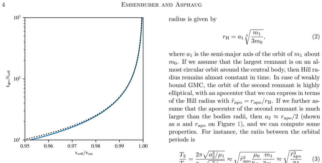
The object that carries the argument is the scaled apocenter distance $\tilde{r}_{\rm apo}=r_{\rm apo}/r_H$, the farthest separation reached by the two post-impact remnants divided by the radius of the larger body's Hill sphere. The machinery is a staged decomposition of a graze-and-merge collision: the first impact is treated as a hydrodynamical event whose outcome fixes a point-mass orbit, then a hybrid symplectic N-body integrator with direct close-encounter handling evolves that orbit under the central body for 10,000 randomly oriented realisations per configuration, and the second collision is sampled from the resulting encounters. The authors anchor the decomposition by checking one SPH simulation, finding that the relative motion is well described by two-body dynamics once the remnants separate beyond about six mutual radii. A period-ratio estimate, $T_2/T_1\approx\sqrt{\tilde{r}_{\rm apo}^3/24}$, shows that the relative motion of the central body during the loop-back depends only on orientation and $\tilde{r}_{\rm apo}$, which motivates the scale invariance and the use of the Hill radius as the natural yardstick.
What would settle it
Run the paper's Monte Carlo setup with the post-impact apocenter fixed at $\tilde{r}_{\rm apo}=0.5$ but with the target moved from 1 AU to 0.5 AU (or the body radii changed so $\tilde{r}_{\rm coll}$ stays fixed); if the cumulative distribution of delays between the two collisions differs measurably from the paper's $\tilde{r}_{\rm apo}=0.5$ curve, the claimed scale invariance in $\tilde{r}_{\rm apo}$ is wrong. A full SPH simulation with the same first-impact outcome and an explicit third body would also settle whether the point-mass approximation between collisions holds at apocenters in the $0.3$\textendash$0.75$ Hill-radius range.
Extended reading notes
Core claim
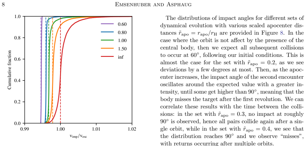
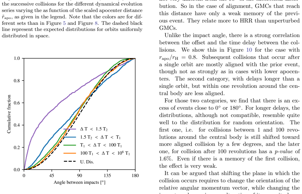
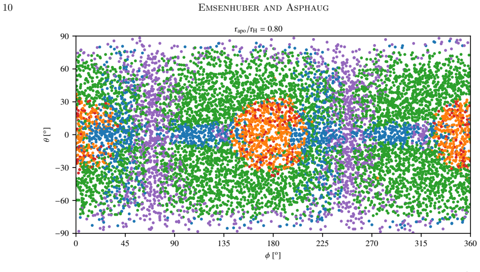
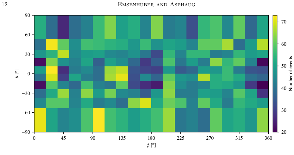
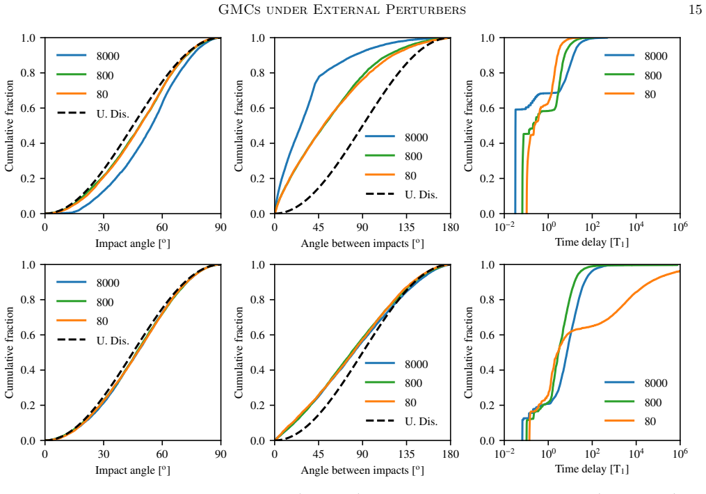
The central claim is that the outcome of a graze-and-merge collision around a third body is governed primarily by the scaled apocenter distance $\tilde{r}_{\rm apo}=r_{\rm apo}/r_H$, the farthest point of the loop-back orbit divided by the Hill radius. The paper's Monte Carlo integrations show that if $\tilde{r}_{\rm apo}\lesssim 0.3$, every realisation returns and collides again after a single orbit, with the second impact nearly aligned with the first. From about one-third to three-quarters of the Hill radius, the central body perturbs the orbit enough that a growing share of realisations miss on the first return, and the distributions of return velocity, impact angle, and orbital-plane alignment drift toward what would be expected for randomly oriented encounters; at $\tilde{r}_{\rm apo}=1.0$ the impact-angle distribution resembles but is not identical to the uniform one, while in the parabolic limit it is statistically indistinguishable from it. Beyond about $\tilde{r}_{\rm apo}\simeq 0.75$, most pairs no longer follow the first impact's geometry and some become unbound, so the process behaves more like a hit-and-run collision than a merger. The paper argues the dependence is scale-free, with a secondary correction encoded by the approximate relation $k\approx \tilde{r}_{\rm apo}-0.2\log_{10}(\tilde{r}_{\rm coll})$, where $\tilde{r}_{\rm coll}=r_{\rm coll}/r_H$, so results obtained for an Earth-like target at 1 AU transfer, within the model's assumptions, to Titan around Saturn and other systems.
Load-bearing premise
The load-bearing premise is that a graze-and-merge collision can be split into independent stages, with the interval between the two collisions governed purely by point-mass gravity; this was checked with only one SPH simulation, and the authors concede it may fail when the Hill sphere is not much larger than the colliding bodies.
Editorial extensions
If this is right
- Graze-and-merge collisions with post-impact apocenters inside about $0.3\,r_H$ can be modelled as isolated two-body mergers without meaningful error.
- For apocenters between roughly $0.3\,r_H$ and $0.75\,r_H$, the second impact must be treated as a random or distribution-sampled event, not as a deterministic consequence of the first collision.
- Accretion scaling laws that count every bound post-impact pair as a merger overestimate growth when the loop-back orbit approaches or exceeds the Hill radius, because a substantial fraction of those pairs either collide only after long chaotic delays or become unbound.
- The Titan moon-formation scenario in which Saturn's middle-sized moons are produced during Titan's accretion is the most affected application: the modelled grazing collisions reach about half of Titan's Hill radius, so Saturn's tides make them hit-and-run events rather than mergers, which reshapes the predicted moon-forming mass budget.
- N-body planet-formation codes should reinsert the bound but widely ranging remnants of a first impact into the integration, treating the graze-and-merge to hit-and-run transition as smooth rather than as a yes/no accretion criterion.
Reading between the lines
- Because the paper fixes the first impact angle at $60^\circ$, a natural extension is to vary impact angle and check whether the outcome map indeed shifts with $\tilde{r}_{\rm coll}$ as the eccentricity argument suggests: more grazing angles should behave like effectively larger $\tilde{r}_{\rm coll}$, and more head-on angles like smaller ones.
- The two-variable scaling $k\approx \tilde{r}_{\rm apo}-0.2\log_{10}(\tilde{r}_{\rm coll})$ is presented as a rough fit; a higher-resolution survey of the $\tilde{r}_{\rm apo}$–$\tilde{r}_{\rm coll}$ plane could test whether a single contour of $k$ really collapses the return-time, impact-angle, and alignment distributions, or whether the fit underestimates early returns at low $\tilde{r}_{\rm apo}
- The same Hill-scaled apocenter criterion could be applied to satellite-accretion and binary-asteroid settings, since the scale-invariance argument is general, but the validation rests on a single SPH simulation, so the transfer of thresholds to settings where the Hill sphere is only a few body radii wide remains to be verified.
- A practical follow-up would be to convert the return-time and impact-property distributions into a simple parametrized return-probability function of $\tilde{r}_{\rm apo}$ and $\tilde{r}_{\rm coll}$ for use in giant-impact population synthesis.
Signed reviews
Editorial analysis
A structured set of objections, weighed in public.
Referee Report
Summary. The paper studies the intermediate orbital phase of graze-and-merge collisions (GMCs) when the colliding pair orbits a third, more massive body. The authors replace the hydrodynamical post-impact evolution with point-mass N-body integrations in the Mercury code, drawing initial conditions from the expected outcome of the first collision: two remnants separated by twice their mutual radii, with the unperturbed return impact angle fixed at 60 degrees and the unperturbed apocenter scaled by the Hill radius. A Monte Carlo procedure samples 10,000 orientations of the post-impact orbit for each apocenter value. The main results are that the standard single-orbit GMC picture holds only for apocenters within about 0.3 r_H, that between roughly 1/3 and 3/4 r_H the return geometry is progressively randomized while the pair still generally re-collides, and that beyond about 3/4 r_H most realizations no longer return on the first orbit and some become unbound. The paper also presents a scaling relation in Eq. (6) involving the apocenter-to-Hill-radius ratio and the body-size-to-Hill-radius ratio, and applies the results to argue that the Asphaug and Reufer (2013) Titan formation scenario is significantly affected by Saturn's presence.
Significance. If the thresholds and scaling relation hold, the paper makes a useful contribution to planet and satellite formation: it shows that GMCs cannot always be treated as isolated two-body mergers, identifies a smooth transition between GMC and hit-and-run regimes, and provides a cheap N-body methodology for exploring the intermediate orbit. The Monte Carlo strategy is efficient, the scale-invariance argument in Section 3 is clearly motivated, and the main thresholds are supported by the cumulative distributions in Figures 5-9. The paper also offers falsifiable predictions: the 0.3 r_H and 0.75 r_H transitions could be tested with dedicated hydrodynamical simulations. However, the current validation of the central separability assumption is thin, and the paper's strongest astrophysical conclusion about the Titan scenario rests on that assumption in a regime where it is least tested.
major comments (4)
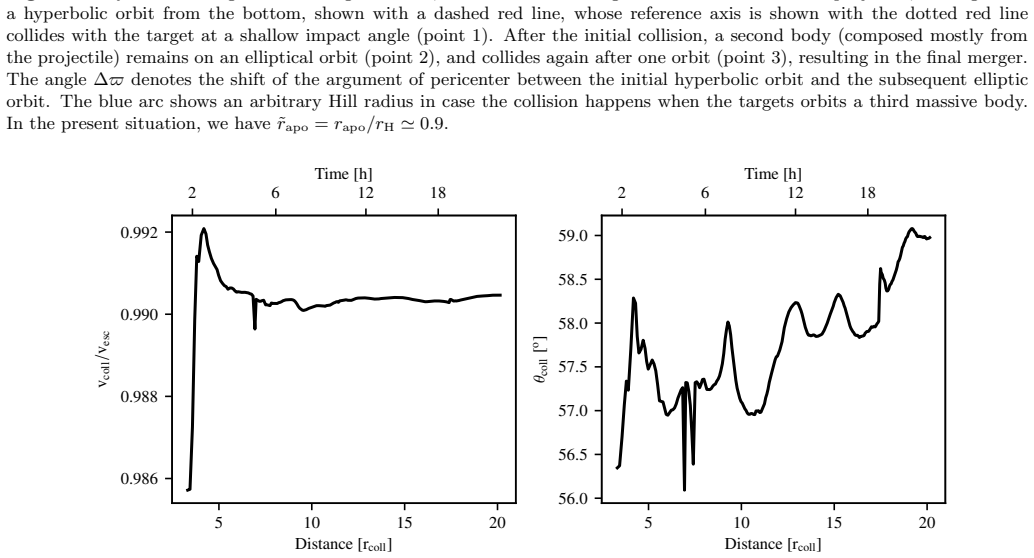
- [Sections 2 and 4; Section 7.4] The separability assumption is validated by only one SPH simulation, and that validation does not cover the initial conditions actually used in the main suite. Section 2 finds that two-body behavior begins only after the remnants separate by about six mutual radii, yet Section 4 starts the N-body integrations with the bodies separated by twice their mutual radii. The interval from 2 to 6 r_coll is therefore treated as point-mass dynamics without direct support. This is not a purely academic concern: for the Titan application in Section 7.3, r_H/r_coll is about 12.6 and r_apo ~ 0.5 r_H corresponds to only about 6.3 r_coll, so the entire modeled intermediate orbit lies at the edge of the validated regime. Section 7.4 itself concedes that separability 'might not be entirely correct when the Hill radius is not much larger than the body sizes.' I ask the authors to either add SPH validation for other impact angles, mass ratios, and smaller r_H/r_coll values, or clearly restrict the claims to the validated regime and soften the Titan conclusion accordingly.
- [Section 4 and Section 6.2] The main suite fixes the unperturbed return impact angle at 60 degrees, and the paper provides no N-body series with different impact angles. Section 6.2 states that the results 'slightly depend on the choice of the impact angle' and even predicts the direction of the shift for grazing versus more head-on collisions, but no simulations are shown. Since the impact angle controls the pericenter-to-rcoll relationship and hence the orbital eccentricity, the central thresholds at 0.3 r_H and 0.75 r_H, as well as the scaling relation in Eq. (6), are established for a single geometry. The generality claims in Section 7.1 therefore go beyond what is demonstrated. A small number of additional series with, for example, 30 and 80 degree return angles would make the parameter dependence quantitative.
- [Abstract versus Section 5.1 and Section 7.1] The abstract states that when the loop-back orbit reaches about 3/4 of the Hill radius, the smaller body 'will usually escape the target.' This is not what the simulations show. Section 5.1 reports that for r_apo/r_H = 1.0 more than 90% of realizations collide within 1e6 T1, and even the parabolic limiting case has a return rate above 80% within 1e6 T1. Section 7.1 more carefully states only that 'some of the pairs get unbound.' The abstract should be reworded to match the actual results, for example by saying that most realizations no longer return after a single orbit and a minority become unbound.
- [Section 7.3] The claim that the specific Asphaug and Reufer (2013) Titan collisions 'are not, in fact, accretionary, but should be counted as hit and run' is stronger than the presented simulations justify. The N-body runs use a 60 degree return angle and a mass ratio gamma = 0.1, which are not shown to match the A&R collision parameters. Moreover, at r_apo/r_H ~ 0.5, the paper's own Figure 6 indicates that a substantial fraction of realizations still return after a single orbit, and Section 5.1 shows that all pairs at this apocenter collide within 100 T1. The conclusion may be correct, but as written it overreaches; rephrasing to say that the A&R scenario is 'likely to be significantly perturbed' or 'needs to be re-evaluated' would be more appropriate unless A&R-like initial conditions are explicitly simulated.
minor comments (6)
- [Table 1] There are typos in Table 1: 'Merucry' should be 'Mercury,' and the table header 'T able 1' has an extra space.
- [Figure 4 caption] The caption contains a duplicated word: 'the plane denotes denotes the orbital planet of m1 about m0'; also 'planet' should presumably be 'plane.'
- [Section 5.2.2] The legend text 'Note that the colors are for different sets than in Figures 5 or 5' should refer to the correct companion figure (probably Figure 7), not repeat Figure 5.
- [Section 6.1] In the discussion of rtilde_coll = 0.1, the text refers to 'the lower boundary on Figure 6,' but the relevant panel is Figure 14, which plots the r_H/r_coll axis; Figure 6 has r_apo/r_H on the horizontal axis.
- [Section 5.2.1] The word 'apoceneters' is a typo for 'apocenters.'
- [Section 7.2] There is a duplicated 'where' in the sentence beginning 'For instance, in the case where where rtilde_coll = 0.1...'
Circularity Check
No significant circularity: the 1/3 and 3/4 Hill-radius thresholds emerge from N-body integrations, not from the fitted scaling law or from self-citations.
full rationale
The paper's central claims are the return-time, impact-angle, and alignment transitions near 1/3 and 3/4 of the Hill radius. These are outputs of 10,000-realisation Mercury N-body integrations with apocenter distance as the controlled input and uniformly random orbital orientations; they are read off cumulative distributions in Figures 5, 6, 8, and 9, and are not imposed by any equation. The initial conditions deliberately fix the unperturbed return angle at 60 degrees, so the low-apocenter agreement with 60 degrees is a consistency check of the numerical setup, not a derived prediction; the physically meaningful result is the progressive randomisation at larger apocenter, which is not in the initial conditions. Equation (6) is explicitly introduced as a rough fit to reproduce Figure 6, and is then tested on independent N-body sets with different r_H/r_coll values in Section 6.2 (Figure 15), so it is a fitted scaling relation with validation rather than a fitted input renamed as a prediction. Self-citations to EA19 are used for one SPH validation run, the bound-remnant search, the Monte Carlo procedure, and contextual comparison of return rates; none of these is load-bearing for the main thresholds. The staged-separability assumption is stated openly and its limitation is conceded in Section 7.4, which is an acknowledged scope restriction rather than a circular argument. Overall, the derivation chain is self-contained with respect to the central claim; the minor non-load-bearing self-citations do not make it circular.
Assumptions & free parameters
free parameters (3)
- Reference return impact angle =
60 degrees
- Remnant mass ratio m2/m1 =
0.1
- Scaling coefficient in Eq. (6) =
0.2
assumptions (5)
- ad hoc to paper A GMC can be divided into independent stages, with point-mass two-body dynamics applying once the remnants are separated by about six mutual radii.
- domain assumption The post-encounter orbit is fully described by an apocenter set to a fraction of the Hill radius and a pericenter that would produce a 60-degree impact angle in the unperturbed case, with the orientation distributed uniformly on a sphere.
- domain assumption The largest remnant moves on a circular orbit around the central body so that the Hill radius is constant in time.
- domain assumption Mercury's hybrid symplectic and Bulirsch-Stoer integration accurately tracks close encounters over up to 10^6 orbital periods.
- standard math Keplerian two-body dynamics and energy conservation give the correct unperturbed mapping between impact velocity, apocenter, and period ratio.
Cite this review
Pith. "Pith review of Graze-and-Merge Collisions under External Perturbers." pith.science (2026). https://pith.science/paper/VUCUKJ64
@misc{pith2026190807557,
  author       = {Pith},
  title        = {Pith review of: Graze-and-Merge Collisions under External Perturbers},
  year         = {2026},
  howpublished = {\url{https://pith.science/paper/VUCUKJ64}},
  note         = {Machine review of arXiv:1908.07557}
}
read the original abstract
Graze-and-merge collisions (GMCs) are common multi-step mergers occurring in low-velocity off-axis impacts between similar sized planetary bodies. The first impact happens at somewhat faster than the mutual escape velocity; for typical impact angles this does not result in immediate accretion, but the smaller body is slowed down so that it loops back around and collides again, ultimately accreting. The scenario changes in the presence of a third major body, i.e. planets accreting around a star, or satellites around a planet. We find that when the loop-back orbit remains inside roughly 1/3 of the Hill radius from the target, then the overall process is not strongly affected. As the loop-back orbit increases in radius, the return velocity and angle of the second collision become increasingly random, with no record of the first collision's orientation. When the loop-back orbit gets to about 3/4 of the Hill radius, the path of smaller body is disturbed up to the point that it will usually escape the target.
Figures

Figures from the paper (12 more)






Reference graph
Works this paper leans on
-
[1]
, " * write output.state after.block = add.period write newline
ENTRY address archivePrefix author booktitle chapter doi edition editor eprint howpublished institution journal key month number organization pages publisher school series title misctitle type volume year version url label extra.label sort.label short.list INTEGERS output.state before.all mid.sentence after.sentence after.block FUNCTION init.state.consts ...
-
[2]
write newline
" write newline "" before.all 'output.state := FUNCTION format.url url empty "" new.block "" url * "" * if FUNCTION format.eprint eprint empty "" archivePrefix empty "" archivePrefix "arXiv" = new.block " " eprint * " " * new.block " " eprint * " " * if if if FUNCTION format.doi doi empty "" " " doi * " " * if FUNCTION format.pid doi empty eprint empty ""...
-
[3]
sj c ; HR3c= cg 96m nI] XPHٛڤ ^QFXv z|e
thebibliography [1] 20pt to REFERENCES 6pt =0pt 10pt plus 3pt =0pt =0pt =1pt plus 1pt =0pt =0pt -12pt =13pt plus 1pt =20pt =13pt plus 1pt \@M =10000 =-1.0em =0pt =0pt 0pt =0pt =1.0em @enumiv\@empty 10000 10000 `\.\@m \@noitemerr \@latex@warning Empty `thebibliography' environment \@ifnextchar \@reference \@latexerr Missing key on reference command Each re...
2017
-
[4]
Agnor , C. B., Canup , R. M., & Levison , H. F. 1999, , 142, 219, 10.1006/icar.1999.6201
arXiv 1999
-
[5]
2010, Chemie der Erde / Geochemistry, 70, 199, 10.1016/j.chemer.2010.01.004
Asphaug , E. 2010, Chemie der Erde / Geochemistry, 70, 199, 10.1016/j.chemer.2010.01.004
-
[6]
Asphaug , E., Agnor , C. B., & Williams , Q. 2006, , 439, 155, 10.1038/nature04311
-
[7]
2013, , 223, 544, 10.1016/j.icarus.2012.12.009
Asphaug , E., & Reufer , A. 2013, , 223, 544, 10.1016/j.icarus.2012.12.009
-
[8]
Benz , W., Slattery , W. L., & Cameron , A. G. W. 1986, , 66, 515, 10.1016/0019-1035(86)90088-6
Show all 26 references
-
[9]
Canup , R. M. 2004, , 168, 433, 10.1016/j.icarus.2003.09.028
2004 doi
- [10]
-
[11]
2011, , 141, 35, 10.1088/0004-6256/141/2/35
---. 2011, , 141, 35, 10.1088/0004-6256/141/2/35
2011 doi
-
[12]
M., & Asphaug , E
Canup , R. M., & Asphaug , E. 2001, , 412, 708
2001
-
[13]
Chambers , J. E. 1999, , 304, 793, 10.1046/j.1365-8711.1999.02379.x
1999
-
[14]
2013, , 224, 43, 10.1016/j.icarus.2013.02.015
---. 2013, , 224, 43, 10.1016/j.icarus.2013.02.015
2013 doi
-
[15]
1969, Ellipsoidal figures of equilibrium (New Haven: Yale University Press)
Chandrasekhar , S. 1969, Ellipsoidal figures of equilibrium (New Haven: Yale University Press)
1969
-
[16]
2019, , 875, 95, 10.3847/1538-4357/ab0c1d
Emsenhuber , A., & Asphaug , E. 2019, , 875, 95, 10.3847/1538-4357/ab0c1d
2019 doi
-
[17]
Hunter , J. D. 2007, Computing in Science and Engineering, 9, 90, 10.1109/MCSE.2007.55
2007 doi
-
[18]
2010, , 714, L21, 10.1088/2041-8205/714/1/L21
Kokubo , E., & Genda , H. 2010, , 714, L21, 10.1088/2041-8205/714/1/L21
2010 doi
-
[19]
2007, , 671, 2082, 10.1086/522364
Kokubo , E., & Ida , S. 2007, , 671, 2082, 10.1086/522364
2007 doi
-
[20]
M., Marcus , R
Leinhardt , Z. M., Marcus , R. A., & Stewart , S. T. 2010, , 714, 1789, 10.1088/0004-637X/714/2/1789
2010 doi
-
[21]
M., & Stewart , S
Leinhardt , Z. M., & Stewart , S. T. 2012, , 745, 79, 10.1088/0004-637X/745/1/79
2012 doi
-
[22]
2018, , 2, 555, 10.1038/s41550-018-0471-7
Leleu , A., Jutzi , M., & Rubin , M. 2018, , 2, 555, 10.1038/s41550-018-0471-7
2018 doi
-
[23]
Sanz-Serna, J. M. 1992, Acta Numerica, 1, 243–286, 10.1017/S0962492900002282
1992 doi
-
[24]
Shoemaker, E. M. 1962, in Physics and Astronomy of the Moon, ed. Z. Kopal (Academic Press, New York), 283--359
1962
-
[25]
T., & Leinhardt , Z
Stewart , S. T., & Leinhardt , Z. M. 2012, , 751, 32, 10.1088/0004-637X/751/1/32
2012 doi
-
[26]
1980, Introduction to Numerical Analysis (Springer-Verlag, New York)
Stoer , J., & Bulirsch , R. 1980, Introduction to Numerical Analysis (Springer-Verlag, New York)
1980
Reviewed August 14, 2026 · model on record in the stance chip above.
Discussion (0). Continue with ORCID to comment.