REVIEW 5 major objections 9 minor 82 references
Self-Sustained Oscillations of a Nonlinear Optomechanical System in the Low-Excitation Regime
T0 review · 5 major / 9 minor · reviewed 2026-08-04 · deepseek-v4-flash
Pith's one-line read A Kerr-nonlinear superconducting optomechanical circuit undergoes mechanical self-oscillation at few-photon cavity occupancy, with a parameter-free semi-classical model reproducing the measured response.
desk verdict Solid experimental demonstration of self-sustained oscillations at few-photon occupations in a Kerr optomechanical device, but the abstract's 'four orders of magnitude' and 'single-excitation' claims do not survive contact with the paper's own numbers. read the letter →
The pith
A machine-rendered reading of the paper's core claim, the machinery that carries it, and where it could break.
The reading
The authors compare their measurements to two calculations: an analytical model of the scattering response in stable and unstable regions, and a numerical integration of the classical equations of motion. The parameters---cavity loss, Kerr strength, mechanical frequency, damping, and optomechanical coupling---were measured beforehand in separate low-power calibration experiments and then entered without fitting. Across three device settings and a wide range of powers, the numerical curves match the data, including the blue-sideband dips. At the highest settings a quick frequency sweep reveals extra sidebands, but the pulsed steady-state protocol removes those transient features and restores agreement with the model.
Extended reading notes
Core claim
The central claim, stated in the abstract, is: "we report the observation and theoretical modeling of nonlinear dynamics in a mechanical system driven at the single-excitation level" and that "the large Kerr nonlinearity of our superconducting microwave circuit reduces the threshold for the observation of nonlinear dynamics by four orders of magnitude, making this regime experimentally accessible at the few-photon level." If the paper is correct, the device exhibits genuine self-sustained mechanical oscillations at intra-cavity photon numbers of order 1-100, and the observed scattering response is quantitatively reproduced by a semi-classical model with independently measured parameters, not by fitting the nonlinear data.
Load-bearing premise
The absolute photon-number calibration supports the few-photon claim. In Appendix D, the drive power at the sample is inferred from EMIT fits that assume linear-regime operation (K n_bar_c ≈ 0) and use a g0 value determined from temperature-dependent sideband spectroscopy. If that calibration were off, every threshold reported in units of photons (n_in/n_in,crit, n_bar_c ≈ 2-120) would shift, and the "single-excitation level" or "four orders of magnitude" statements would lose their quantitative meaning. This is load-bearing for the central quantitative claim and is distinct from the physical identification of the sideband dips as self-sustained oscillations.
Signed reviews
Editorial analysis
A structured set of objections, weighed in public.
Referee Report
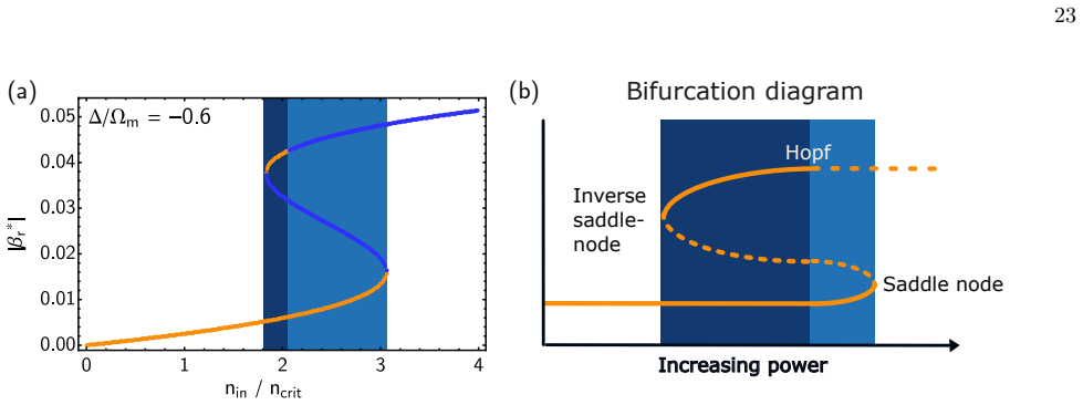
Summary. The paper reports measurements of a superconducting microwave optomechanical device with an intrinsic Kerr nonlinearity, operated with a pulsed single-tone scattering protocol. It observes a power- and detuning-dependent deformation of the cavity resonance and an additional absorption dip near the blue sideband, attributed to self-sustained mechanical oscillations (Hopf instability). The authors model the response with a semi-classical Hamiltonian including Kerr and optomechanical coupling, analyze the fixed-point stability diagram (Figs. 2, 13–15), derive analytical scattering formulas for stable (Eq. 2) and unstable (Eq. 3) regimes with a power-balance closure (Eqs. H18–H22), and validate against time-domain numerical integration of the classical equations of motion (Appendix H2). System parameters are independently calibrated: circle fitting for κ and K, sideband spectroscopy for Ωm and Γm, EMIT and temperature-dependent sideband areas for g0, and an EMIT-based input-line attenuation for absolute photon numbers (Appendices C, D). Agreement is shown for three parameter sets over many powers (Fig. 4) and in the SI for a fourth set (Fig. 10). The central abstract claim is that the Kerr nonlinearity reduces the threshold for nonlinear dynamics by four orders of magnitude, accessing the few-photon regime with intra-cavity occupations n̄c ≈ 2–120.
Significance. If correct, the paper's contribution is substantial: it presents a parameter-free, independently calibrated semi-classical model that quantitatively reproduces a complex nonlinear optomechanical scattering response across several parameter sets, and it places the onset of mechanical self-oscillation at intra-cavity photon numbers of order 1–100, far below typical optomechanical instability thresholds. The machine-readable data/code and the pulsed protocol that suppresses transient artifacts are clear strengths, as is the cross-validation of g0 and photon calibration by two independent methods. The benchmark in Appendix G, however, uses the linear-cavity formula (Eq. G1) for the instability threshold, which is inconsistent with the proposed Kerr-enabled mechanism emphasized in the abstract and Fig. 2. The main quantitative claim about 'four orders of magnitude' reduction is fragile: it conflates the cavity bistability (saddle-node) threshold with the mechanical self-oscillation (Hopf) threshold, and for the latter the Kerr nonlinearity does not reduce but rather raises the threshold relative to a linear cavity with the same parameters. This distinction is load-bearing for the abstra
major comments (5)
- [Abstract, Fig. 2, Table I caption] The 'four orders of magnitude' claim conflates two different thresholds. n_in,crit introduced in Fig. 2 is the saddle-node (bistability) threshold n_in,crit = 2κ³/(3√3κ_ext K_eff) (Eq. H11), with n̄_c,crit = κ/√(3K_eff) ≈ 19 for set III. But the observed feature attributed to self-sustained oscillations is the Hopf instability, not bistability. For a linear cavity (K=0) with the same Table I parameters, the standard optomechanical instability threshold at Δ=Ω_m is n̄_c,th ≈ Γ_m κ/(4g0²) ≈ 0.3 for set III, corresponding to n_in,th ≈ 8×10^7 s^-1 ≈ -154 dBm, roughly 34 dB below the -120 dBm quoted as the Kerr-lowered threshold. Thus the Kerr nonlinearity raises the power required for the observed Hopf instability relative to K=0; the 'four orders' statement is only defensible for the Duffing-like bistability of the cavity photon branches, a different observable. The abstract and Fig. 2 shou
- [Appendix G, Eq. G1] Appendix G explicitly uses the linear-cavity formula n̄_c(Γ_opt=-Γ_m) = (1+n̄_m,lin)/C_0 to benchmark 'our device' against previous works, and states that 'the threshold is only marginally influenced by the Kerr nonlinearity.' This contradicts the paper's central mechanism claim that the Kerr nonlinearity enables the low-excitation regime, and it undermines the benchmark's validity: if the Kerr effect is crucial, then the comparison should use the actual Hopf threshold for the nonlinear system, not the linear formula. Moreover, Fig. 11 claims the device is the first to reach a quantum-nonlinear-mechanics region, but that claim relies on the disputed threshold calculation and on Eq. G2, whose derivation and assumptions are not given in the main text/SI. Either provide the nonlinear-system derivation of both G1 and G2 and the corresponding threshold values, or soften the benchmark claims t
- [Appendix D, Eqs. C6, D3] The absolute photon-number calibration is load-bearing for the few-photon claim. The input-line attenuation is inferred from EMIT fits that assume linear-regime operation (K n̄_c ≈ 0) and use g0 from temperature-dependent sideband spectroscopy. Eq. C6 is the linear-cavity photon number formula; if the drive power used in the EMIT calibration is not fully in the linear regime, or if g0 itself is slightly biased by the Kerr-shifted operating point, the inferred attenuation and all quoted n̄_c values (2–120) would shift. The manuscript reports statistical uncertainties on the attenuation (54.4±0.3 dB) and on g0 (e.g., ±0.07 kHz), but does not estimate the systematic error from the linear-regime assumption (K n̄_c ≈ 0) in the calibration. Please add a quantitative estimate of this systematic uncertainty (e.g., the largest K n̄_c/K consistent with the EMIT data) and state how it propagates to
- [Eq. (H13) and text after] The derivation of the scattering formula in the stable regime is not fully clear. Starting from Eq. H12, which is the response of a two-tone (pump-probe) scheme with probe frequency ω, the text says 'we remove the second weak probe tone ... by setting its frequency to zero' to obtain Eq. H13. Setting ω=0 in Eq. H12 gives the pump's own response, which is not the same as the standard single-tone input-output result if the pump itself is part of the nonlinear steady state. Eq. H13 uses n̄_c determined from Eq. H10, which is the steady-state photon number of the driven nonlinear cavity; this is plausible, but the claim that it is 'obtained' by setting ω=0 should be justified more carefully, since the linearized small-probe susceptibility is not Eq. H12 with ω=0. If this is merely a heuristic steady-state identification, state so and check that Eq. H13 reproduces the low-power limit correctl
- [Abstract and Discussion] The paper's claim of 'single-excitation level' or 'few-photon level' is based on the steady-state photon number n̄_c ≈ 2–120. However, the observed mechanical self-oscillation is a classical limit cycle with large mechanical amplitude; the photon occupation during the oscillation includes multi-photon sidebands (Bessel-function components), and the quantum/non-classical content of the state is not addressed. The abstract's 'single-excitation level' phrasing is likely to be read as a single quanta of excitation of the mechanical system, which is not what is measured. Please clarify in the abstract and introduction whether 'single-excitation level' refers to the intra-cavity photon occupation of the drive tone (a classical amplitude), not to the mechanical oscillator's quantum state, and consider using 'few-photon drive level' to avoid overclaiming.
minor comments (9)
- [Eq. (3)] Eq. (3) has a typo: the Bessel product is written J_n(z1)J_n(z1); presumably this is J_n(z1)². The SI version (Eq. H17) has the same notation; please fix.
- [Fig. 2 and text] The caption says 'panel c extends a to vastly larger input powers. Only then one can observe multi-stability in a linear system'; this is the point of the 'four orders' claim, but the y-axis normalization uses n_in,crit for the Kerr system, which makes the comparison hard to read. Consider also plotting absolute input photon flux.
- [Table I / Fig. 4] The main text refers to 'parameter set I' in the SI; the caption of Fig. 3 says 'for parameter set III' but the paper's discussion of Fig. 3d says 'above bifurcation' — clarify which set is used in each panel. Also, the caption says 'n_in/n_in,crit = 0.008 and 1.10' but the text says '−118.6 dBm' for 1.10; the conversion to dBm is given only once, which makes it hard to verify the quoted numbers.
- [Sec. II B] The notation n̄_c,crit = κ/√(3K_eff) is stated in Table I; the definition of Δ_crit is not stated in the main text. Use consistent notation and point to the SI for the derivation.
- [References] Ref. [58] (Probst) is a resonant absorption calibration reference; the circle-fitting method is cited, but the specific 'modified circle fitting algorithm' is described only in the SI. That is fine, but the main text should note that the algorithm is detailed in Appendix C1.
- [Eq. H21 vs Eq. H17] The sign convention of Δ in Eq. H17 is written −i(Δ+K_eff n̄_c − n Ω_m) but the analogous term in Eq. H15 has (+ n Ω_m) in the denominator. Check the sign consistency between the time-domain ansatz (Eq. H14, e^{-iΩ_m t}) and the resulting S21 expression, as a sign error here would flip the sidebands.
- [Sec. III (Discussion)] The text says 'n̄_c ≈ 2−120' but Table I lists n̄_c,crit = 1.6 for set IV; reconcile these values (the range presumably includes off-critical detunings). State whether n̄_c is the steady-state mean at the operating point of the dip or the maximal value over the scan.
- [Eq. G2] The expression for n̄_m,min is quoted without derivation. If it is a known result from Ref. [43], cite it directly; otherwise, provide a derivation in the SI.
- [Appendix E] The transient-response discussion is important and well done. However, the attribution of the extra dips to 'transient dynamics' is only supported by sweep-direction asymmetry; consider adding a sentence that the numerical simulation shown in Fig. 9 is the steady-state model, not a time-dependent simulation including the finite ring-down, to avoid confusion.
Circularity Check
No significant circularity in the central claim; one minor self-consistency check of the Kerr calibration is circular but not load-bearing.
-
other
[Appendix C 1, Eqs. (C2)-(C3) and Fig. 5b,c]
"the circle-fitting routine is adapted to incorporate the Kerr nonlinearity by iteratively optimizing K such that it correctly describes the induced frequency shift ... The cavity response calculated in this way, based on the fit results, is shown in Fig. 5c. It shows excellent agreement with the corresponding experimental data in Fig. 5b. The apparent excellent agreement between theory and experiment validates the value of the Kerr nonlinearity K obtained by the fit."
K is obtained by fitting the power-dependent frequency shift and lineshape of the very data shown in Fig. 5b; the 'validation' in Fig. 5c is the same model evaluated with that fitted K against the same data. It is therefore a self-consistency check, not an independent confirmation. This is not load-bearing for the main result, since the nonlinear scattering data of Figs. 3-4 are compared with K as a fixed input and are not refitted.
full rationale
The central derivation chain is self-contained: the system parameters (κint, κext, K, g0, Ωm, Γm) are determined by separate calibration protocols and then entered as fixed inputs into the analytical and numerical model. The stability analysis and the scattering response in the unstable regime are derived from the Hamiltonian in Appendix H using standard input-output theory, fixed-point analysis, and the power-balance condition Γm + Γopt = 0; they are not obtained by fitting the nonlinear scattering data. The observed blue-sideband absorption dip and its power dependence are compared with the simulation without refitting, so the main 'prediction' is not equivalent to its inputs by construction. The cited overlap with Ref. [43] (same theory group) is not load-bearing because the effective-Kerr and critical-power formulas are re-derived in the appendices and also cite independent sources [54,74]. The one genuinely circular element is the Kerr calibration check in Appendix C: K is extracted from the power-dependent cavity response and then 'validated' by calculating that same response from the fitted K, which is a self-consistency check rather than an independent prediction. This does not undermine the main quantitative comparison. The skeptical concern about the 'four orders of magnitude' statement is a substantive correctness issue, not circularity: the quoted n_in,crit is the Kerr-cavity bifurcation threshold, whereas a linear cavity's self-oscillation threshold can be lower; however, that is a mismatch of definitions and physics, not a derivation that reduces to its own inputs.
Assumptions & free parameters
free parameters (5)
- g0 (single-photon optomechanical coupling) =
4.69 ± 0.07 kHz (set III); 0.76-18.4 kHz across sets
- K (intrinsic Kerr nonlinearity) =
70 kHz (set III); 16 kHz to 1.4 MHz across sets
- κ_int, κ_ext =
e.g. 0.68 MHz and 1.64 MHz (set III)
- Γ_m (mechanical damping rate) =
12 ± 4 Hz (set III)
- Input line attenuation =
54.4 ± 0.3 dB
assumptions (5)
- standard math Standard input-output theory (Gardiner-Collett) gives the classical equations of motion for the cavity and mechanical mode.
- domain assumption During parameter calibration the cavity is operated in its linear response regime, i.e. K n_bar_c ≈ 0.
- domain assumption The mechanical mode thermalizes with the cryostat stage (T_cryo = T_m) for the temperature-dependent sideband calibration.
- domain assumption In the unstable regime the mechanical oscillator executes a single-frequency limit cycle, β = β_bar + B e^{-iΩ_m t} e^{-iφ}.
- standard math The mechanical Kerr contribution K_m = 2 g0^2 Ω_m / (Ω_m^2 + Γ_m^2/4) and the total Kerr K_eff = K + K_m describe the effective cavity nonlinearity.
Cite this review
Pith. "Pith review of Self-Sustained Oscillations of a Nonlinear Optomechanical System in the Low-Excitation Regime." pith.science (2026). https://pith.science/paper/VWK3YUMI
@misc{pith2026251001775,
  author       = {Pith},
  title        = {Pith review of: Self-Sustained Oscillations of a Nonlinear Optomechanical System in the Low-Excitation Regime},
  year         = {2026},
  howpublished = {\url{https://pith.science/paper/VWK3YUMI}},
  note         = {Machine review of arXiv:2510.01775}
}
read the original abstract
Manifesting across all time, mass and length scales, nonlinearities lie at the core of numerous physical phenomena. Next-generation quantum applications, such as quantum sensing, require the combination of nonlinearity with non-classical correlations. This necessitates the search for an experimental platform which enables a nonlinear response at ultra-low excitation levels in a system with practical sensing potential and quantum compatibility. Here, we report the observation and theoretical modeling of nonlinear dynamics in a mechanical system driven at the single-excitation level. We achieve this using a cavity-optomechanical platform with large single-photon coupling rates and a nonlinear microwave resonator. Specifically, the large Kerr nonlinearity of our superconducting microwave circuit reduces the threshold for the observation of nonlinear dynamics by four orders of magnitude, making this regime experimentally accessible at the few-photon level. The parameter-based quantitative predicative power of the theoretical description underlines our deep understanding of the physics involved and that this device concept paves the way for experiments with non-classical microwave drive schemes.
Figures


Figures from the paper (12 more)




Reference graph
Works this paper leans on
-
[1]
Howard and N
L. Howard and N. Kopell,The Hopf Bifurcation and Its Applications, Vol. 19 (Springer, New York, 1976)
1976
-
[2]
Bakemeier, A
L. Bakemeier, A. Alvermann, and H. Fehske, Phys. Rev. Lett.114, 013601 (2015). 7
2015
-
[3]
X.-Y. L¨ u, H. Jing, J.-Y. Ma, and Y. Wu, Phys. Rev. Lett. 114, 253601 (2015)
2015
-
[4]
R. V. Jensen, Phys. Rev. E58, R6907 (1998)
1998
-
[5]
Amitai, N
E. Amitai, N. L¨ orch, A. Nunnenkamp, S. Walter, and C. Bruder, Phys. Rev. A95, 053858 (2017)
2017
-
[6]
Dykman,Fluctuating Nonlinear Oscillators: From Nanomechanics to Quantum Superconducting Circuits (Oxford University Press, 2012)
M. Dykman,Fluctuating Nonlinear Oscillators: From Nanomechanics to Quantum Superconducting Circuits (Oxford University Press, 2012)
2012
-
[7]
Strogatz,Nonlinear dynamics and chaos: with appli- cations to physics, biology, chemistry, and engineering (CRC Press, 2019)
S. Strogatz,Nonlinear dynamics and chaos: with appli- cations to physics, biology, chemistry, and engineering (CRC Press, 2019)
2019
-
[8]
Yurke and D
B. Yurke and D. Stoler, Phys. Rev. Lett.57, 13 (1986)
1986
Show all 82 references
-
[9]
Hofheinz, H
M. Hofheinz, H. Wang, M. Ansmann, R. C. Bialczak, E. Lucero, M. Neeley, A. D. O’Connell, D. Sank, J. Wen- ner, J. M. Martinis, and A. N. Cleland, Nature459, 546 (2009)
2009
-
[10]
Vlastakis, G
B. Vlastakis, G. Kirchmair, Z. Leghtas, S. E. Nigg, L. Frunzio, S. M. Girvin, M. Mirrahimi, M. H. Devoret, and R. J. Schoelkopf, Science342, 607 (2013)
2013
-
[11]
S. Puri, S. Boutin, and A. Blais, npj Quantum Inf.3, 1 (2017)
2017
-
[12]
X. L. He, Y. Lu, D. Q. Bao, H. Xue, W. B. Jiang, Z. Wang, A. F. Roudsari, P. Delsing, J. S. Tsai, and Z. R. Lin, Nat. Commun.14, 6358 (2023)
2023
-
[13]
Aspelmeyer, T
M. Aspelmeyer, T. J. Kippenberg, and F. Marquardt, Rev. Mod. Phys.86, 1391 (2014)
2014
-
[14]
Barzanjeh, A
S. Barzanjeh, A. Xuereb, S. Gr¨ oblacher, M. Paternostro, C. A. Regal, and E. M. Weig, Nat. Phys.18, 15 (2022)
2022
-
[15]
Metcalfe, Appl
M. Metcalfe, Appl. Phys. Rev.1, 031105 (2014)
2014
-
[16]
B. Li, L. Ou, Y. Lei, and Y. Liu, Nanophotonics10, 2799 (2021)
2021
-
[17]
Brennecke, S
F. Brennecke, S. Ritter, T. Donner, and T. Esslinger, Science322, 235 (2008)
2008
-
[18]
L. S. Collaboration and V. Collaboration, Phys. Rev. Lett.116, 061102 (2016)
2016
-
[19]
J. Chan, T. P. M. Alegre, A. H. Safavi-Naeini, J. T. Hill, A. Krause, S. Gr¨ oblacher, M. Aspelmeyer, and O. Painter, Nature478, 89 (2011)
2011
-
[20]
A. D. O’Connell, M. Hofheinz, M. Ansmann, R. C. Bial- czak, M. Lenander, E. Lucero, M. Neeley, D. Sank, H. Wang, M. Weides, J. Wenner, J. M. Martinis, and A. N. Cleland, Nature464, 697 (2010)
2010
-
[21]
J. D. Teufel, T. Donner, D. Li, J. W. Harlow, M. S. All- man, K. Cicak, A. J. Sirois, J. D. Whittaker, K. W. Lehn- ert, and R. W. Simmonds, Nature475, 359 (2011)
2011
-
[22]
E. E. Wollmann, C. U. Lei, A. J. Weinstein, J. Suh, A. Kronwald, F. Marquardt, A. A. Clerk, and K. C. Schwab, Science349, 952 (2015)
2015
-
[23]
Pirkkalainen, E
J.-M. Pirkkalainen, E. Damsk¨ agg, M. Brandt, F. Mas- sel, and M. A. Sillanp¨ a¨ a, Phys. Rev. Lett.115, 243601 (2015)
2015
-
[24]
Barzanjeh, E
S. Barzanjeh, E. S. Redchenko, M. Peruzzo, M. Wulf, D. P. Lewis, G. Arnold, and J. M. Fink, Nature570, 480 (2019)
2019
-
[25]
Lecocq, J
F. Lecocq, J. B.Clark, R. W. Simmonds, J. Aumentado, and J. D. Teufel, Phys. Rev. X5, 041037 (2015)
2015
-
[26]
Barzanjeh, M
S. Barzanjeh, M. Wulf, M. Peruzzo, M. Kalaee, P. B. Dieterle, O. Painter, and J. M. Fink, Nat Commun8, 953 (2017)
2017
-
[27]
J. S. Huber, G. Rastelli, M. J. Seitner, J. K¨ olbl, W. Belzig, M. I. Dykman, and E. M. Weig, Phys. Rev. X10, 021066 (2020)
2020
-
[28]
J. S. Ochs, D. K. J. Boneß, G. Rastelli, M. Seitner, W. Belzig, M. I. Dykman, and E. M. Weig, Phys. Rev. X12, 041019 (2022)
2022
-
[29]
Kuang, R
T. Kuang, R. Huang, W. Xiong, Y. Zuo, X. Han, F. Nori, C. Qiu, H. Luo, H. Jing, and G. Xiao, Nat. Phys.19, 414 (2023)
2023
-
[30]
A. A. Clerk, F. Marquardt, and J. G. E. Harris, Phys. Rev. Lett.104, 213603 (2010)
2010
-
[31]
xi Liu, A
Y. xi Liu, A. Miranowicz, Y. B. Gao, J. Bajer, C. P. Sun, and F. Nori, Phys. Rev. A82, 032101 (2010)
2010
-
[32]
Nunnenkamp, K
A. Nunnenkamp, K. Børkje, and S. M. Girvin, Phys. Rev. Lett.107, 063602 (2011)
2011
-
[33]
Rabl, Phys
P. Rabl, Phys. Rev. Lett.107, 063601 (2011)
2011
-
[34]
J. Qian, A. A. Clerk, K. Hammerer, and F. Marquardt, Phys. Rev. Lett.109, 253601 (2012)
2012
-
[35]
Kronwald and F
A. Kronwald and F. Marquardt, Phys. Rev. Lett.111, 133601 (2013)
2013
-
[36]
P. D. Nation, Phys. Rev. A88, 053828 (2013)
2013
-
[37]
B. D. Hauer, A. Metelmann, and J. P. Davis, Phys. Rev. A98, 043804 (2018)
2018
-
[38]
B. D. Hauer, J. Combes, and J. D. Teufel, Phys. Rev. Lett.130, 213604 (2023)
2023
-
[39]
Schmidt, M
P. Schmidt, M. T. Amawi, S. Pogorzalek, F. Deppe, A. Marx, R. Gross, and H. Huebl, Commun. Phys.3, 1 (2020)
2020
-
[40]
I. C. Rodrigues, D. Bothner, and G. A. Steele, Nat Com- mun10, 5359 (2019)
2019
-
[41]
Zoepfl, M
D. Zoepfl, M. L. Juan, N. Diaz-Naufal, C. M. F. Schnei- der, L. F. Deeg, A. Sharafiev, A. Metelmann, and G. Kirchmair, Phys. Rev. Lett.130, 033601 (2023)
2023
-
[42]
T. Bera, S. Majumder, S. K. Sahu, and V. Singh, Com- mun Phys4, 1 (2021)
2021
-
[43]
Diaz-Naufal, L
N. Diaz-Naufal, L. Deeg, D. Zoepfl, C. M. F. Schneider, M. L. Juan, G. Kirchmair, and A. Metelmann, Phys. Rev. A111, 053505 (2025)
2025
-
[44]
Bothner, I
D. Bothner, I. C. Rodrigues, and G. A. Steele, Commun Phys5, 1 (2022)
2022
-
[45]
Majumder, T
S. Majumder, T. Bera, and V. Singh, Phys. Rev. Res.4, 033232 (2022)
2022
-
[46]
L. F. Deeg, D. Zoepfl, N. Diaz-Naufal, M. L. Juan, A. Metelmann, and G. Kirchmair, Phys. Rev. Appl.23, 014082 (2025)
2025
-
[47]
Carmon, H
T. Carmon, H. Rokhsari, L. Yang, T. J. Kippenberg, and K. J. Vahala, Phys. Rev. Lett.94, 223902 (2005)
2005
-
[48]
Marquardt, J
F. Marquardt, J. G. E. Harris, and S. M. Girvin, Phys. Rev. Lett.96, 103901 (2006)
2006
-
[49]
A. G. Krause, J. T. Hill, M. Ludwig, A. H. Safavi-Naeini, J. Chan, F. Marquardt, and O. Painter, Phys. Rev. Lett. 115, 233601 (2015)
2015
-
[50]
S. R. Das, S. Majumder, S. K. Sahu, U. Singhal, T. Bera, and V. Singh, Phys. Rev. Lett.131, 067001 (2023)
2023
-
[51]
Luschmann, P
T. Luschmann, P. Schmidt, F. Deppe, A. Marx, A. Sanchez, R. Gross, and H. Huebl, Sci. Rep.12, 1608 (2022)
2022
-
[52]
P. D. Nation, M. P. Blencowe, and E. Buks, Phys. Rev. B78, 104516 (2008)
2008
-
[53]
T. F. Roque, New J. Phys22, 013049 (2020)
2020
-
[54]
Aldana, C
S. Aldana, C. Bruder, and A. Nunnenkamp, Phys. Rev. A88, 043826 (2013)
2013
-
[55]
C. W. Gardiner and M. J. Collett, Phys. Rev. A31, 3761 (1985)
1985
-
[56]
Ludwig, B
M. Ludwig, B. Kubala, and F. Marquardt, New Journal of Physics10, 095013 (2008)
2008
-
[57]
C. L. Degen, F. Reinhard, and P. Cappellaro, Rev. Mod. Phys.89, 035002 (2017). 8
2017
-
[58]
Probst, F
S. Probst, F. B. Song, P. A. Bushev, A. V. Ustinov, and M. Weides, Rev. Sci. Instrum.86, 024706 (2015)
2015
-
[59]
M. S. Khalil, M. J. A. Stoutimore, F. C. Wellstood, and K. D. Osborn, J. Appl. Phys.111, 054510 (2012)
2012
-
[60]
Rieger, S
D. Rieger, S. G¨ unzler, M. Spiecker, A. Nambisan, W. Wernsdorfer, and I. Pop, Phys. Rev. Appl.20, 014059 (2023)
2023
-
[61]
M. L. Gorodetksy, A. Schliesser, G. Anetsberger, S. Deleglise, and T. J. Kippenberg, Opt. Express18, 23236 (2010)
2010
-
[62]
S. Weis, R. Rivi` ere, S. Del´ eglise, E. Gavartin, O. Arcizet, A. Schliesser, and T. J. Kippenberg, Science330, 1520 (2010)
2010
-
[63]
X. Zhou, F. Hocke, A. Schliesser, A. Marx, H. Huebl, R. Gross, and T. J. Kippenberg, Nature Phys.9, 179 (2013)
2013
-
[64]
Singh, S
V. Singh, S. J. Bosman, B. H. Schneider, Y. M. Blanter, A. Castellanos-Gomez, and G. A. Steele, Nature Nan- otech9, 820 (2014)
2014
-
[65]
J. D. Teufel, D. Li, M. S. Allman, K. Cicak, A. J. Sirois, J. D. Whittaker, and R. W. Simmonds, Nature471, 204 (2011)
2011
-
[66]
Bruno, G
A. Bruno, G. De Lange, S. Asaad, K. L. Van Der Enden, N. K. Langford, and L. DiCarlo, Appl. Phys. Lett.106, 182601 (2015)
2015
-
[67]
Schmidt, D
P. Schmidt, D. Schwienbacher, M. Pernpeintner, F. Wulschner, F. Deppe, A. Marx, R. Gross, and H. Huebl, Appl. Phys. Lett.113, 152601 (2018)
2018
-
[68]
C. A. Regal, J. D. Teufel, and K. W. Lehnert, Nature Phys4, 555–560 (2008)
2008
-
[69]
Weber, J
P. Weber, J. G¨ uttinger, A. Noury, J. Vergara-Cruz, and A. Bachtold, Nat Commun7, 12496 (2016)
2016
-
[70]
Doolin, B
C. Doolin, B. D. Hauer, P. H. Kim, A. J. R. MacDon- ald, H. Ramp, and J. P. Davis, Phys. Rev. A89, 053838 (2014)
2014
-
[71]
T. Bera, M. Kandpal, G. S. Agarwal, and V. Singh, Nat Commun15, 7115 (2024)
2024
-
[72]
Delattre, I
A. Delattre, I. Golokolenov, R. Pedurand, X. Zhou, A. Fefferman, and E. Collin, Phys. Rev. Res.6, 043038 (2024)
2024
-
[73]
H. Wang, S. Singh, C. R. H. McRae, J. C. Bardin, S.-X. Lin, N. Messaoudi, A. R. Castelli, Y. J. Rosen, E. T. Hol- land, D. P. Pappas, and J. Y. Mutus, Quantum Science and Technology6, 035015 (2021)
2021
-
[74]
Laflamme and A
C. Laflamme and A. A. Clerk, Phys. Rev. A83, 033803 (2011)
2011
-
[75]
A. D. Armour and D. A. Rodrigues, Comptes Ren- dus Physique13, 440 (2012), advances in nano- electromechanical systems
2012
-
[76]
D. A. Rodrigues and A. D. Armour, Phys. Rev. Lett. 104, 053601 (2010)
2010
-
[77]
Ludwig,Collective quantum effects in optomechanical systems, Ph.D
M. Ludwig,Collective quantum effects in optomechanical systems, Ph.D. thesis, Friedrich-Alexander-Universit¨ at Erlangen-N¨ urnberg (F AU) (2013). 9 Appendix A: Device F abrication The device is structured on a high-resistivity silicon wafer (R >10 kΩ cm), from which a 6 by 10...
2013
-
[78]
This is done using a modified circle fitting algorithm, based on the methods presented in Refs
Cavity Parameters Before any other system parameters can be determined, it is essential to first characterize the cavity. This is done using a modified circle fitting algorithm, based on the methods presented in Refs. [46, 58], which also allows for the extraction of the Kerr ...
-
[79]
In this technique, a continuous-wave drive is applied to the microwave cavity, and the resulting first-order mechanical sidebands are analyzed
Mechanical Parameters The mechanical frequency Ωm, decay rate Γm, and quality factorQ m are determined through sideband spectroscopy. In this technique, a continuous-wave drive is applied to the microwave cavity, and the resulting first-order mechanical sidebands are analyzed....
-
[80]
In essence, by applying a sideband drive, a transparency window is created within the cavity resonance, whose amplitude depends ong 0
Single-Photon Coupling Rate In this section, we explain how the single-photon coupling rateg 0 can be determined through electromechanically- induced transparency (EMIT) [40, 62–64]. In essence, by applying a sideband drive, a transparency window is created within the cavity r...
-
[81]
Analytics Using the Hamiltonian given in Eq. H2, we obtain the following equations of motion for the cavity and mechanical mode using standard input-output theory [55], d dt ˆa=i∆ˆa− κ 2 ˆa+iKˆa†ˆaˆa−ig0ˆa(ˆb+ ˆb†)− r κext 2 αp − √κˆain,(H3) d dt ˆb=−(iΩ m + Γm 2 )ˆb−ig 0ˆa†ˆa...
-
[82]
We start with the nonlinear equations of motion given in Eqs
Simulation An alternative route to obtain the cavity response is to numerically solve the equations of motion and use the standard input-output relation. We start with the nonlinear equations of motion given in Eqs. H5 and H6, and rewrite them in terms of the real and imaginar...
Reviewed August 4, 2026 · model on record in the stance chip above.
Discussion (0). Continue with ORCID to comment.