REVIEW 4 major objections 4 minor 57 references
Quantum-Enhanced Simulated Annealing Using Rydberg Atoms
T0 review · 4 major / 4 minor · reviewed 2026-08-07 · deepseek-v4-flash
Pith's one-line read Quantum-prepared warm starts let simulated annealing solve larger maximum-independent-set graphs, up to 8,655 vertices, within a one-day classical runtime.
desk verdict A useful experimental demonstration of warm-started SA on Rydberg MIS graphs, undermined by an inconsistent fitting formula and an extrapolation that outruns the evidence. read the letter →
The pith
A machine-rendered reading of the paper's core claim, the machinery that carries it, and where it could break.
The reading
What carries the argument
The load-bearing object is the epoch-performance ratio $y(\mathrm{HD}/N) = 1/[c_1(\exp(\beta \,\mathrm{HD}/N)-1)]$, with $c_1=0.1602$ and $\beta=6.738$, which turns a warm start's normalized Hamming distance into a multiplicative speedup for simulated annealing. It is used with two fitted scaling laws: the epoch-to-solution count $\mathrm{ETS}_{\mathrm{MIS,SA}} = aN e^{b\sqrt{N}}$ for King's-lattice graphs (the graph of legal king moves on a chessboard), and the per-epoch processing time $t_\mathrm{step}=cN^d$. Their product gives the total processing time whose one-day cutoff yields the $N_c$ numbers. The Rydberg experiment's role is to supply a starting configuration with a small $\mathrm{HD}/N$, and the paper's quantitative claim is that this single number, rather than any other property of the quantum state, predicts the speedup.
What would settle it
Compute true MIS sizes for King's-lattice graphs at N = 200, 300, and 500, run QESA and standalone SA to alpha = 0.95, and check whether the epoch ratio still follows y = 1/[0.1602(exp(6.738 HD/N) - 1)] and whether the fitted a, b, c, d coefficients stay constant; if they drift, the one-day N_c values, including 8,655, are not reliable.
Extended reading notes
Core claim
The paper's central claim is that the entire benefit of the quantum warm start can be summarized by the normalized Hamming distance HD/N between the starting spin configuration and the target solution: the closer the quantum experiment puts the SA start to the answer, the fewer epochs SA needs. The authors fit the epoch ratio y = Epoch#(SA)/Epoch#(QESA) to y(HD/N) = 1/[0.1602(exp(6.738 HD/N)-1)] with adjusted $R^{2}$ = 0.9838, and show that the measured AQC and QE points follow this curve. Combining this ratio with the known King's-graph scaling ETS_MIS,SA = aN $e^{{b sqrt N}}$ and the per-epoch time t_step = cN^d, they estimate the largest graph that can be solved within one day on their PC: 5,312 vertices for SA alone, rising to 8,655 when the warm start has HD/N = 0.07. They also note that QESA's occupation-swap update gives a narrower, higher-mean distribution of approximation ratios than the earlier Rydberg post-processing approach.
Load-bearing premise
The load-bearing premise is that the time-to-solution formulas fitted to 60-170-vertex King's-lattice graphs remain accurate up to thousands of vertices, and that a shorter starting Hamming distance fully captures the quantum advantage.
Editorial extensions
If this is right
- If the epoch-ratio model holds, QESA cuts SA time to a target approximation ratio by a factor that grows as HD/N shrinks; the paper measures performance gaps of 1.15, 1.75, 2.63, and 9.94 for HD/N = 0.32, 0.21, 0.15, and 0.07 at alpha = 0.99.
- Within a fixed one-day PC budget, the largest tractable King's-graph MIS instance grows from 5,312 vertices for standalone SA to 5,484, 6,023, 6,584, or 8,655 vertices depending on warm-start quality.
- Both warm-start protocols, adiabatic evolution and quench evolution on a neutral-atom device, give the same qualitative advantage, so the benefit is not tied to one specific quantum control scheme.
- Because QESA includes an occupation-swap move, its final approximation ratios are more concentrated around a higher mean than those of the earlier Rydberg post-processing method.
Reading between the lines
- The model predicts that any warm start with a given normalized Hamming distance, whether produced by a Rydberg experiment, a classical heuristic, or a greedy solver, yields the same SA speedup; this is an untested consequence of reducing the quantum advantage to HD/N alone.
- The paper does not measure whether quantum states carry structural correlations beyond Hamming distance that help SA; comparing QESA to classical warm starts with matched HD/N would isolate any such residual quantum benefit.
- The one-day N_c values extrapolate from N = 170 to thousands of vertices; running the same QESA protocol on intermediate graphs (N = 200-500) with known MIS sizes would show whether the fitted scaling coefficients remain stable.
- Outside King's-lattice unit-disk graphs, the hardness exponent in the ETS formula would likely change, but the QESA warm-start framework should transfer if the appropriate hardness growth is substituted.
Editorial analysis
A structured set of objections, weighed in public.
Referee Report
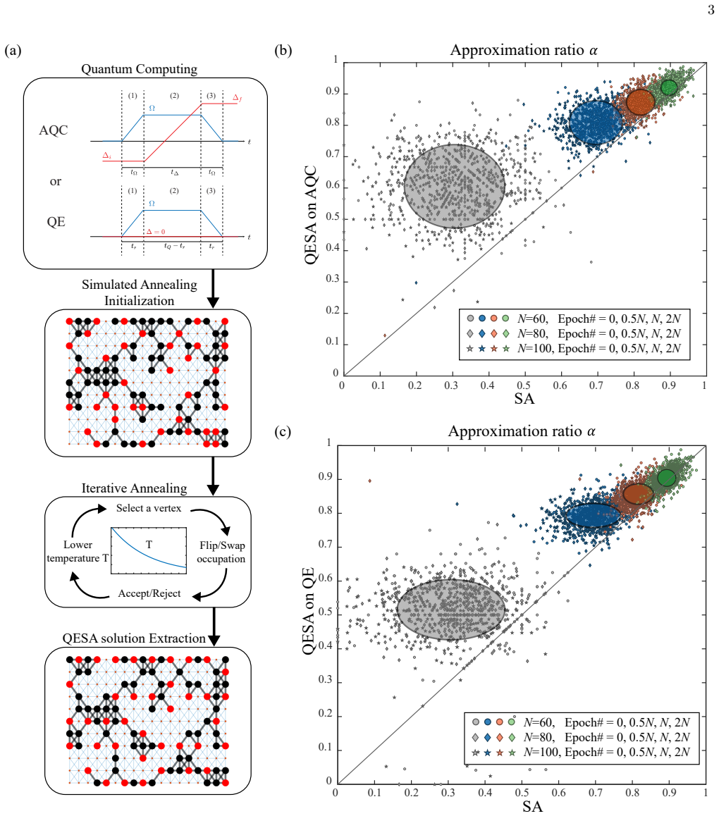
Summary. The paper reports a hybrid quantum-classical algorithm, QESA, for the maximum independent set (MIS) problem. QESA uses measurement outcomes from Rydberg-atom experiments (archived AQC data and new quench-evolution data on QuEra Aquila) as warm-start initial configurations for simulated annealing (SA). The authors compare QESA with random-start SA on King's-lattice graphs with N=60-170, report that a large fraction of instances reach a fixed approximation ratio in fewer SA epochs, fit an empirical relation between the epoch ratio and normalized Hamming distance (Eq. 4), and extrapolate to estimate the maximum graph size solvable within one day on a PC: N_c=8,655 for QESA at HD/N=0.07 versus 5,312 for standalone SA. The data and code are made publicly available.
Significance. The direct experimental comparison is a useful empirical case study: on the tested graphs, warm-starting SA from Rydberg measurements reduces the number of epochs needed to reach alpha_t=0.95 compared with random-start SA with the same total occupation number. The public release of data, code, and figures is a strength. However, the quantitative model that converts this observation into a projected N_c is not currently supported. The fitted equation (Eq. 4) is inconsistent with the values used in the extrapolation (Fig. 3), the advantage is attributed entirely to Hamming distance without a classical warm-start control, and the scaling extrapolation from N=60-170 to N~8,700 is unvalidated. The 'quantum-enhanced' component of the central claim is therefore not established, even though the paper's direct experimental comparison is not circular.
major comments (4)
- [Section IV, Eq. (4) and Fig. 3 (caption and inset)] The fitted curve y(HD/N)=1/[c1(exp(beta*HD/N)-1)] with c1=0.1602 and beta=6.738 gives y(0.32)=0.82, y(0.21)=2.00, y(0.15)=3.57, and y(0.07)=10.35, whereas Fig. 3 reports performance gaps of 1.15, 1.75, 2.63, and 9.94 for the same HD/N values (and the listed a0/a values are 1, 1.15, 1.74, 2.63, and 9.94). Thus Eq. (4) is not the curve used to produce the headline N_c estimates; at HD/N=0.32, Eq. (4) predicts that QESA is slower than SA (ratio less than 1), yet the paper still lists N_c=5,484 > 5,312 for that case. This internal inconsistency bears directly on the central extrapolation and must be resolved.
- [Section V, first sentence, and Eq. (4)] The paper states that 'QESA is a subset of SA that begins at a shorter Hamming distance' and models the entire QESA advantage through the initial HD/N. No classical warm-start baseline at matched HD/N is provided. The comparisons in Fig. 1(b,c) are against random-start SA with the same total occupation number, which by construction has a larger HD/N. A classical warm start (a greedy MIS heuristic, local search, or a short SA pre-run) that produces the same HD/N distribution would, under the paper's own model, yield the same speedup. Without such a control, the experimental data support only 'warm-started SA beats random-start SA,' not 'quantum-enhanced SA' as the cause of the speedup; the extrapolation to N_c=8,655 and the conclusion of a quantum-originated advantage are therefore not established.
- [Section VI and Fig. 3] The N_c estimates are obtained by extrapolating ETS_{MIS,SA}=aN e^{b sqrt(N)} (Eq. 5) and t_step=cN^d (Eq. 6), with all parameters fitted to graphs with N=60-170, up to N approximately 8,700. No evidence is given that the hardness exponent b=1.0738 or the per-epoch cost exponent d=0.76 remain valid over this 50-fold range. The one-day runtime constraint makes the result very sensitive to small errors in these exponents. The authors should either validate the scaling on larger classical instances or clearly label N_c as a speculative extrapolation rather than an 'expected' capability.
- [Section IV, Hamming distance definition] The target configuration t in the definition HD = |{j: s_j != t_j}| is never specified. It is not stated whether t is the exact MIS solution, the best solution found by SA, or the final QESA solution. The numerical values of HD/N used in Fig. 2 and Fig. 3 depend critically on this choice, and without it the fitted model in Eq. (4) is not reproducible.
minor comments (4)
- [Eq. (7) and Fig. 3 caption] Equation (7) and the caption of Fig. 3 write t_processing = aN x b sqrt(N) x cN^d, but the definition in Eq. (5) is ETS = aN e^{b sqrt(N)}; the exponential factor is missing in Eq. (7) and in the caption. Please correct this typo, since the extrapolated curves depend on the exponential factor.
- [Section IV, after Eq. (3)] The text states that alpha is derived from the MIS Hamiltonian 'with Delta=1 and U=1', while Section III states that U=11 is chosen for King's graphs. Please clarify which value is used in the SA cost function and how alpha relates to the energy when U is not 1.
- [Throughout] The term 'Epoch#' is used repeatedly but never defined; from Fig. 1 it appears that one epoch corresponds to N proposed updates. Please define it explicitly in Section III or IV.
- [Throughout] There are numerous typographical errors (for example, 'indepedent', 'archieved', 'despote', 'probem', 'spead', and 'Natura Phys.') that should be corrected in a revision.
Circularity Check
The headline N_c=8,655 extrapolation is the SA-fitted warm-start curve re-evaluated at smaller HD/N; the direct QESA-vs-SA experiment is not itself circular.
-
fitted input called prediction
[Section IV (Eq. 4) and Section V / Fig. 3 caption (Eqs. 5-7)]
"The required processing time is estimated as aN × b√N × cN^d based on Equation 5 and the epoch performance ratio in Figure 2, where a0 = 5.0508, b= 1.0738, c = 25.44 µs, d = 0.76 and a0/a = 1, 1.15, 1.74, 2.63 and 9.94 for SA and ⟨HD/N⟩ = 0.32, 0.21, 0.15 and 0.07 cases, respectively. From these estimations, the upper bounds Nc of graph size within the one-day limit are predicted to be 5,312 for SA and as 5,484, 6,023, 6,584, and 8,655..."
The 'epoch performance ratio in Figure 2' is Equation 4, fit with c1=0.1602 and β=6.738 to the 'QESA Model', which is constructed by sampling SA spin configurations at initial αi=0.85/0.88/0.91 and sorting their epoch differences by HD. The text then states that a in Eq. 5 is 'inversely proportional to the epoch performance ratio in Equation 4.' Therefore the QESA processing times and all Nc values are obtained by evaluating the SA-fitted exponential curve at smaller HD/N; the extrapolated 8,655-vertex claim is the same SA scaling evaluated with a reduced initial Hamming distance, not an independent quantum-derived prediction.
-
self definitional
[Section V, first paragraph and Eq. 5]
"Since QESA is a subset of SA that begins at a shorter Hamming distance, we analyze its scaling behavior in comparison to that of SA. ... where a is a coefficient associated with the normalized Hamming distance HD/N (inversely proportional to the epoch performance ratio in Equation 4)."
The paper defines QESA's scaling behavior, for the extrapolation, as identical to SA's except for the initial HD/N value. Because the coefficient a in Eq. 5 is set by the SA-fitted ratio from Eq. 4, the predicted quantum advantage is forced, by construction, to equal the classical SA warm-start advantage. Any quantum-originated improvement beyond Hamming distance is excluded from the model, so the reported Nc for QESA is logically just SA's Nc evaluated at smaller fitted HD/N values. The experimental QESA data are real, but the headline projection reduces to a relabeled SA warm-start curve.
full rationale
The direct experimental comparison in Fig. 1 has independent content: 97.5% of AQC-based and 91.9% of QE-based graphs reach αt=0.95 in fewer epochs than standalone SA, and these are genuine measurements. However, the paper's scaling model is circular in a specific, quotable way. Equation 4 fits the epoch ratio y(HD/N)=1/[c1(exp(β·HD/N)-1)] to a 'QESA Model' that is built from SA configurations warmed to αi=0.85/0.88/0.91, not from quantum data. Section V then says QESA 'is a subset of SA that begins at a shorter Hamming distance' and sets the coefficient a in Eq. 5 inversely proportional to the Eq. 4 ratio. The Fig. 3 caption confirms that the Nc estimates are computed 'based on Equation 5 and the epoch performance ratio in Figure 2.' Consequently, the headline projections (Nc up to 8,655) are evaluations of SA's own fitted scaling at smaller HD/N, with the classical warm-start benefit relabeled as quantum enhancement. No classical warm-start baseline at matched HD/N is provided, so the model cannot distinguish quantum-originated advantage from a generic better-start advantage. This is not a self-citation-chain issue: Eqs. 5-6 cite external SA scaling results and PC timing, and the experimental datasets are real. Score 6 reflects that the central empirical comparison is non-circular while the central extrapolated prediction reduces by construction to its fitted inputs.
Assumptions & free parameters
free parameters (6)
- c1 =
0.1602
- beta =
6.738
- a =
5.05, 4.39, 2.89, 1.92, 0.51
- b =
1.0738
- c =
25.44 microseconds
- d =
0.76
assumptions (7)
- domain assumption SA epoch scaling Epoch#(SA) = c1 e^{beta m*} with m* approximated by HD/N
- domain assumption ETS_MIS,SA = a N e^{b sqrt(N)} for King's graphs
- domain assumption Per-epoch time scales as tstep = c N^d
- ad hoc to paper QESA is a subset of SA starting at a shorter Hamming distance
- domain assumption Exact MIS sizes are available for every graph to compute alpha
- standard math Rydberg blockade Hamiltonian maps to the MIS cost function
- standard math Adiabatic theorem ensures a low-energy final state in AQC
Cite this review
Pith. "Pith review of Quantum-Enhanced Simulated Annealing Using Rydberg Atoms." pith.science (2026). https://pith.science/paper/VWM4OPNZ
@misc{pith2026250613264,
  author       = {Pith},
  title        = {Pith review of: Quantum-Enhanced Simulated Annealing Using Rydberg Atoms},
  year         = {2026},
  howpublished = {\url{https://pith.science/paper/VWM4OPNZ}},
  note         = {Machine review of arXiv:2506.13264}
}
read the original abstract
Quantum-classical hybrid algorithms offer a promising strategy for tackling computationally challenging problems, such as the maximum independent set (MIS) problem that plays a crucial role in areas like network design and data analysis. This study experimentally demonstrates that a Rydberg quantum-classical hybrid algorithm, termed as quantum-enhanced simulated annealing (QESA), provides a computational time advantage over standalone simulated annealing (SA), a classical heuristic optimization method. The performance of QESA is evaluated based on the approximation ratio and the Hamming distance, relative to the graph size. The analysis shows that QESA outperforms standalone SA by leveraging a warm-start input derived from two types of Rydberg atomic array experimental data: quench evolution (QE) (implemented on the Quera Aquila machine) and adiabatic quantum computing (AQC) (using the experimental dataset archieved in K. Kim et al., Scientific Data 11, 111 (2024). Based on these results, an estimate is provided for the maximum graph size that can be handled within a one-day computational time limit on a standard personal computer. These findings suggest that QESA has the potential to offer a computational advantage over classical methods for solving complex optimization problems efficiently.
Figures


Reference graph
Works this paper leans on
-
[1]
Simulating physics with computers,
R. P. Feynman, “Simulating physics with computers,” Int. J. Theor. Phys. 21, 467 (1982)
work page 1982
-
[2]
M. A. Nielsen and I. L. Chuang, Quantum Computation and Quantum Information(Cambridge University Press, Cambridge, 2010)
2010
-
[3]
Quantum technology: the second quantum revolution,
J. Dowling and G. Milburn, “Quantum technology: the second quantum revolution,” Phil. Trans. 361, 1655 (2003)
work page 2003
-
[4]
Quantum information with Rydberg atoms,
M. Saffman, T. G. Walker, and K. Mølmer, “Quantum information with Rydberg atoms,” Rev. Mod. Phys. 82, 2313 (2010)
2010
- [5]
-
[6]
Quantum information processing with su- perconducting circuits: a review,
G. Wendin, “Quantum information processing with su- perconducting circuits: a review,” Rep. Prog. Phys.80, 106001 (2017)
work page 2017
-
[7]
Quantum supremacy us- ing a programmable superconducting processor,
F. Arute, K. Arya, R. Babbush, D. Bacon, J. C. Bardin, R. Barends, R. Biswas, S. Boixo, F. G. S. L. Brandao, D. A. Buell, B. Burkett, Y. Chen, Z. Chen, B. Chiaro, R. Collins, W. Courtney, A. Dunsworth, E. Farhi, B. Foxen, A. Fowler, C. Gidney, M. Giustina, R. Graff, K. Guerin, S. Habegger, M. P. Harrigan, M. J. Hartmann, A. Ho, M. Hoffmann, T. Huang, T. S...
work page 2019
-
[8]
C. S. Adams, J. D. Pritchard, and J. P. Shaffer, ‘Rydberg atom quantum technologies,” J. Phys. B: At. Mol. Opt. Phys. 53, 012002 (2020)
work page 2020
Show all 57 references
-
[9]
Quantum computing with atomic qubits and Rydberg interactions: progress and challenges,
M Saffman, “Quantum computing with atomic qubits and Rydberg interactions: progress and challenges,” J. Phys. B: At. Mol. Opt. Phys. 49, 202001 (2016)
2016
-
[10]
Quantum technologies with Rydberg atoms,
S. K. Barik, A. Thakur, Y. Jindal, B. S. Silpa, and S. Roy, “Quantum technologies with Rydberg atoms,” Front. Quantum Sci. Technol. 3, 1426216 (2024)
2024
-
[11]
Quantum simulation and computing with Rydberg-interacting qubits,
M. Morgado and S. Whitlock, “Quantum simulation and computing with Rydberg-interacting qubits,” A VS Quan- tum Sci. 3, 023501 (2021)
2021
-
[12]
Quantum optimization for maximum indepen- dent set using Rydberg atom arrays,
H. Pichler, S.-T. Wang, L. Zhou, S. Choi, and M. D. Lukin, “Quantum optimization for maximum indepen- dent set using Rydberg atom arrays,” arXiv:1808.10816 (2018)
2018 arXiv
-
[13]
Frequency assignment: Theory and appli- cations,
W. K. Hale, “Frequency assignment: Theory and appli- cations,” Proc. IEEE68, 1497 (1980)
1980
-
[14]
Fast and simple approximation algorithms for maxi- mum weighted independent set of links,
P. -J. Wan, X. Jia, G. Dai, H. Du, and O. Frieder, “Fast and simple approximation algorithms for maxi- mum weighted independent set of links,” in IEEE IN- FOCOM 2014 - IEEE Conference on Computer Com- munications, Toronto, ON, Canada, April 2014, 1653, https://doi.org/10.1109/...
2014
-
[15]
Finding a Maximal Weighted Independent Set in Wireless Networks,
S. Basagni, “Finding a Maximal Weighted Independent Set in Wireless Networks,” Telecommunication Systems 18, 155 (2001)
2001
-
[16]
Statistical mechanics of maximal independent sets,
L. Dall’Asta, P. Pin, and A. Ramezanpour, “Statistical mechanics of maximal independent sets,” Phys. Rev. E 80, 061136 (2009)
2009
-
[17]
A Novel Approach for the Process Planning and Scheduling Problem Using the Concept of Maximum Weighted Independent Set,
K. Sun, “A Novel Approach for the Process Planning and Scheduling Problem Using the Concept of Maximum Weighted Independent Set,” arXiv:2008.01960 (2020)
2020 arXiv
-
[18]
A Maximum Indepen- dent Set Method for Scheduling Earth Observing Satel- lite Constellations,
D. Eddy and M. J. Kochenderfer, “A Maximum Indepen- dent Set Method for Scheduling Earth Observing Satel- lite Constellations,” arXiv:2008.08446 (2020)
2020 arXiv
-
[19]
Arora and B
S. Arora and B. Barak, Computational Complexity: A Modern Approach (Cambridge Univ. Press, Cambridge, 2009)
2009
-
[20]
Rydberg quantum wires for maximum independent set problems
M. Kim, K. Kim, J. Hwang, E.-G. Moon, and J. Ahn, “Rydberg quantum wires for maximum independent set problems”, Nature Phys. 18, 755 (2022)
2022
-
[21]
Exploring the impact of graph locality for the resolution of the maximum-independent-set problem with neutral atom devices,
C. Dalyac, L.-P. Henry, M. Kim, J. Ahn, and L. Henriet, “Exploring the impact of graph locality for the resolution of the maximum-independent-set problem with neutral atom devices,” Phys. Rev. A 108, 052323 (2009)
2009
-
[22]
Finding the maxi- mum independent sets of Platonic graphs using Rydberg atoms,
A. Byun, M. Kim, and J. Ahn, “Finding the maxi- mum independent sets of Platonic graphs using Rydberg atoms,” PRX Quantum 3, 030305 (2022)
2022
-
[23]
Jeong, M
S. Jeong, M. Kim, M. Hhan, J. Park, and J. Ahn, ”Quan- tum programming of the satisfiability problem with Ry- dberg atom graphs,” Phys. Rev. Res. 5, 043037 (2023)
2023
-
[24]
Quantum Computing Dataset of Maximum Independent Set Prob- lem on King’s Lattice of over Hundred Rydberg Atoms,
K. Kim, M. Kim, J. Park, A. Byun, J. Ahn, “Quantum Computing Dataset of Maximum Independent Set Prob- lem on King’s Lattice of over Hundred Rydberg Atoms,” Scientific Data 11, 111 (2024)
2024
-
[25]
Rydberg-atom experi- ment for the integer factorization problem,
J. Park, S. Jeong, M. Kim, K. Kim, A. Byun, L. Vignoli, L-P. Henry, L. Henriet, J. Ahn, “Rydberg-atom experi- ment for the integer factorization problem,” Phys. Rev. Res. 6, 023241 (2024)
2024
-
[26]
Quantum optimization of maximum independent set us- ing Rydberg atom arrays,
S. Ebadi A. Keesling, M. Cain, T. T. Wang, H. Levine, D. Bluvstein, G. Semeghini, A. Omran, J.-G. Liu, R. Sama- jdar, X.-Z. Luo, B. Nash, X. Gao, B. Barak, E. Farhi, S. Sachdev, N. Gemelke, L. Zhou, S. Choi, H. Pichler, S.-T. Wang, M. Greiner, V. Vuleti´ c, and M. D. Lukin, “Q...
2022
-
[27]
Quan- tum simulation of Cayley-tree Ising Hamiltonians with three dimensional Rydberg atoms,
Y. Song, M. Kim, H. Hwang, W. Lee, and J. Ahn, “Quan- tum simulation of Cayley-tree Ising Hamiltonians with three dimensional Rydberg atoms,” Phys. Rev. Res. 3, 013286 (2021)
2021
-
[28]
Rydberg-atom graphs for quadratic uncon- strained binary optimization problems,
A. Byun, J. Jung, K. Kim, M. Kim, S. Jeong, H. Jeong, and J. Ahn, “Rydberg-atom graphs for quadratic uncon- strained binary optimization problems,” Adv. Quantum. Technol. 2300398 (2024)
2024
-
[29]
Demonstration of Weighted-Graph Optimization on a Rydberg-Atom Array Using Local Light Shifts
A. G. de Oliveira, E. Diamond-Hitchcock, D. M. Walker, M. T. Wells-Pestell, G. Pelegr ´ ı, C. J. Picken, G. P. A. Malcolm, A. J. Daley, J. Bass, and J. D. Pritchard, “Demonstration of Weighted-Graph Optimization on a Rydberg-Atom Array Using Local Light Shifts” PRX Quantum 6, ...
2025
-
[30]
The theory of variational hybrid quantum- classical algorithms
J. R. McClean, J. Romero, R. Babbush, and A. Aspuru- Guzik, “The theory of variational hybrid quantum- classical algorithms” New J. Phys. 18, 023023 (2016)
2016
-
[31]
Solving Nonna- tive Combinatorial Optimization Problems Using Hybrid Quantum–Classical Algorithms,
J. Wurtz, S. H. Sack, and S.-T. Wang, “Solving Nonna- tive Combinatorial Optimization Problems Using Hybrid Quantum–Classical Algorithms,” IEEE Transactions on Quantum Engineering 5, 1 (2024)
2024
-
[32]
Aquila: QuEra’s 256-qubit neutral-atom quantum com- puter,
J. Wurtz, A. Bylinskii, B. Braverman, J. Amato-Grill, S. H. Cantu, F. Huber, A. Lukin, F. Liu, P. Wein- berg, J. Long, S.-T. Wang, N. Gemelke, and A. Keesling, “Aquila: QuEra’s 256-qubit neutral-atom quantum com- puter,” arXiv:2306.11727 (2023)
2023 arXiv
-
[33]
Programming higher- order interactions of Rydberg atoms,
A. Byun, S. Jeong, and J. Ahn, “Programming higher- order interactions of Rydberg atoms,” Phys. Rev. A 110, 042612 (2024)
2024
-
[34]
Photon recoil and laser focusing limits to Rydberg gate fidelity,
F. Robicheaux, T. M. Graham, and M. Saffman, “Photon recoil and laser focusing limits to Rydberg gate fidelity,” Phys. Rev. A 103, 022424 (2021)
2021
-
[35]
Effect of laser-frequency fluc- tuation on the decay rate of Rydberg coherence,
B. Kim, K.-T. Chen, C.-Y. Hsu, S.-S. Hsiao, Y.-C. Tseng, C.-Y. Lee, S.-L. Liang, Y.-H. Lai, J. Ruseckas, G. Juzeli¯ unas, and I. A. Yu, “Effect of laser-frequency fluc- tuation on the decay rate of Rydberg coherence,” Phys. Rev. A 100, 013815 (2019)
2019
-
[36]
Computing Solution Space Properties of Com- binatorial Optimization Problems Via Generic Tensor Networks,
J.-G. Liu, X. Gao, M. Cain, M. D. Lukin, and S.-T. Wang, “Computing Solution Space Properties of Com- binatorial Optimization Problems Via Generic Tensor Networks,” SIAM Journal on Scientific Computing 45, A1239 (2023)
2023
-
[37]
Quantum phases of matter on a 256-atom programmable quantum simulator,
S. Ebadi, T. T. Wang, H. Levine, A. Keesling, G. Se- meghini, A. Omran, D. Bluvstein, R. Samajdar, H. Pich- ler, W. W. Ho, S. Choi, S. Sachdev, M. Greiner, V. Vuleti´ c, and M. D. Lukin, “Quantum phases of matter on a 256-atom programmable quantum simulator,” Nature 595, 227 (2021)
2021
-
[38]
How to Build a Quantum Super- computer:Scaling from Hundreds to Millions of Qubits,
M. Mohseni, A. Scherer, K. G. Johnson, O. Wertheim, M. Otten, N. A. Aadit,Y. Alexeev, K. M. Bresniker, K. Y. Camsari, B. Chapman, S. Chatterjee, G. A. Dag- 9 new, A. Esposito, F. Fahim, M. Fiorentino, A. Gajjar, A. Khalid, X. Kong, B. Kulchytskyy, E. Kyoseva, R. Li, P. A. Lott...
2025 arXiv
-
[39]
Approximating Max- imum Independent Set on Rydberg Atom Arrays Using Local Detunings,
H. Yeo, H. E. Kim, and K. Jeong, “Approximating Max- imum Independent Set on Rydberg Atom Arrays Using Local Detunings,” Adv. Quantum Technol. 8, 8, 2400291 (2025)
2025
-
[40]
Quantum Optimization with Arbitrary Connectivity Using Rydberg Atom Arrays,
M.-T. Nguyen, J.-G. Liu, J. Wurtz, M. D. Lukin, S.- T. Wang, and H. Pichler, “Quantum Optimization with Arbitrary Connectivity Using Rydberg Atom Arrays,” PRX Quantum 4, 4, 010316 (2023)
2023
-
[41]
Hardness of the maximum-independent-set problem on unit-disk graphs and prospects for quantum speedups,
R. S. Andrist, M. J. A. Schuetz, P. Minssen, R. Yalovet- zky, S. Chakrabarti, D. Herman, N. Kumar, G. Salton, R. Shaydulin, Y. Sun, M.Pistoia, and H. G. Katzgraber, “Hardness of the maximum-independent-set problem on unit-disk graphs and prospects for quantum speedups,” Phys. ...
2023
-
[42]
Probing for Quantum Speed up in Spin- Glass Problems with Planted Solutions,
I. Hen, J. Job, T. Albash, T. F. Rønnow, M. Troyer, and D. A. Lidar, “Probing for Quantum Speed up in Spin- Glass Problems with Planted Solutions,” Phys. Rev. A 92, 042325 (2015)
2015
-
[43]
Performance of a Quantum Annealer on Range-Limited Constraint Sat- isfaction Problems,
A. D. King, T. Lanting, and R. Harris, “Performance of a Quantum Annealer on Range-Limited Constraint Sat- isfaction Problems,” arXiv:1502.02098 (2015)
2015 arXiv
-
[44]
Perspectives of quantum annealing: methods and implementations,
P. Hauke, H. G. Katzgraber, W. Lechner, H. Nishimori, and W. D. Oliver, “Perspectives of quantum annealing: methods and implementations,” Rep. Prog. Phys. 83, 054401 (2020)
2020
-
[45]
Defining and Detecting Quantum Speed up,
T. F. Rønnow, Z. Wang, J. Job, S. Boixo, S. V. Isakov, D. Wecker, J. M. Martinis, D. A. Lidar, and M. Troyer, “Defining and Detecting Quantum Speed up,” Science 345, 420 (2014)
2014
-
[46]
Circumventing superexponen- tial runtimes for hard instancesof quantum adiabatic op- timization,
B. F. Schiffer, D. S. Wild, N. Maskara, M. Cain, M. D. Lukin, and R. Samajdar, “Circumventing superexponen- tial runtimes for hard instancesof quantum adiabatic op- timization,” Phys. Rev. Res. 6, 013271 (2024)
2024
-
[47]
Equation of State Calculations by Fast Computing Machines,
N. Metropolis, A. W. Rosenbluth, M. N. Rosenbluth, A. H. Teller, and E. Teller, “Equation of State Calculations by Fast Computing Machines,” J. Chem. Phys. 21, 1087 (1963)
1963
-
[48]
Monte Carlo sampling methods using Markov chains and their applications,
W. K. Hastings, “Monte Carlo sampling methods using Markov chains and their applications,” Biometrika 57, 97 (1970)
1970
-
[49]
A Novel Wrapped Feature Selection Framework for Devel- oping Power System Intrusion Detection Based on Ma- chine Learning Methods,
Y. Han, Y. Wang, Y. Cao, Z. Geng, and Q. Zhu, “A Novel Wrapped Feature Selection Framework for Devel- oping Power System Intrusion Detection Based on Ma- chine Learning Methods,” IEEE Transactions on Sys- tems, Man, and Cybernetics: Systems 53, 7066 (2023)
2023
-
[50]
Effective Covering Array Generation Using an Improved Particle Swarm Optimization,
Z. Li, Y. Chen, Y. Song, K. Lu, and J. Shen, “Effective Covering Array Generation Using an Improved Particle Swarm Optimization,” IEEE Transactions on Reliability 71, 284 (2022)
2022
-
[51]
Multi-Objective Particle Swarm Optimization Based on Fuzzy Optimality,
Y. Shen and G. Ge, “Multi-Objective Particle Swarm Optimization Based on Fuzzy Optimality,” IEEE Access 7, 101513 (2019)
2019
-
[52]
Iordan, ‘A Comparative Study of Three Heuristic Functions Used to Solve the 8-Puzzle,” Journal of Ad- vances in Mathematics and Computer Science 16(1), 1 (2016)
A.-E. Iordan, ‘A Comparative Study of Three Heuristic Functions Used to Solve the 8-Puzzle,” Journal of Ad- vances in Mathematics and Computer Science 16(1), 1 (2016)
2016
-
[53]
On the Hamming distance in combinatorial optimiza- tion problems on hypergraph matchings,
A. Kammerdiner, P. A. Krokhmal, and P. M. Pardalos, “On the Hamming distance in combinatorial optimiza- tion problems on hypergraph matchings,” Opt. Lett. 4, 609 (2010)
2010
-
[54]
Cooling Schedules for Optimal Annealing,
B. Hajek, “Cooling Schedules for Optimal Annealing,” Math. Oper. Res. 13, 311 (1988)
1988
-
[55]
Convergence Rate of a Simu- lated Annealing Algorithm with Noisy Observations,
C. Bouttier and I. Gavra, “Convergence Rate of a Simu- lated Annealing Algorithm with Noisy Observations,” J. Mach. Learn. Res. 20, 1 (2019)
2019
-
[56]
Demonstration of a Scal- ing Advantage for a Quantum Annealer over Simulated Annealing,
T. Albash and D. A. Lidar, “Demonstration of a Scal- ing Advantage for a Quantum Annealer over Simulated Annealing,” Phys. Rev. X 8, 031016 (2018)
2018
-
[57]
Codes, Data and Figures for “Quantum-enhanced simulated annealing using Rydberg atoms,
S. Jeong, J. Park, and J. Ahn, “Codes, Data and Figures for “Quantum-enhanced simulated annealing using Rydberg atoms,” https://doi.org/10.6084/m9.figshare.c.7639259.v1
Reviewed August 7, 2026 · model on record in the stance chip above.
Discussion (0). Sign in to comment.