REVIEW 2 major objections 5 minor 49 references
The assembly of freely moving rigid fibers measures the flow gradient tensor
T0 review · 2 major / 5 minor · reviewed 2026-08-14 · deepseek-v4-flash
Pith's one-line read Rigid fibers can reconstruct the whole flow gradient tensor
desk verdict The 2D fiber-assembly gradient measurement is a solid numerical proof-of-concept, but the 3D claim in the title and abstract is both unverified and, with the stated projection, mathematically impossible. read the letter →
The pith
A machine-rendered reading of the paper's core claim, the machinery that carries it, and where it could break.
The reading
What carries the argument
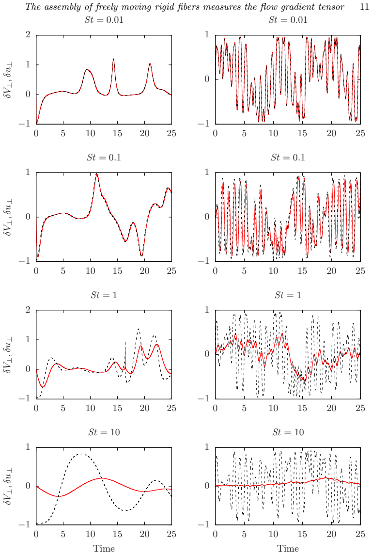
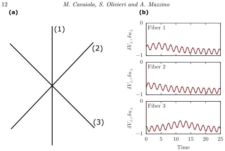
The load-bearing object is the normal-projected end-to-end velocity difference of a single fiber. Writing $\hat{\mathbf r}$ for the fiber orientation and $\hat{\mathbf r}_\perp$ for a normal direction, the paper defines $\delta V_\perp = \delta\mathbf V\cdot\hat{\mathbf r}_\perp$ and $\delta u_\perp = \delta\mathbf u\cdot\hat{\mathbf r}_\perp$, and shows numerically that $\delta V_\perp \approx \delta u_\perp$ at small Stokes number. The tangential component is killed by inextensibility, so the usable signal lives in the normal direction. For short fibers, $\delta u_\perp \approx D = \partial_j u_i\,\hat r_j\,\hat r_{\perp i}$, so each fiber provides one linear equation in the unknown gradient. An assembly of $N_f$ fibers with distinct orientations forms the linear system (Eq. 3.9) that is solved for $\partial_j u_i$; the two-dimensional incompressible case requires three fibers, and the three-dimensional case requires eight.
What would settle it
Place a rigid fiber with rotational Stokes number $St \ll 1$ and length much smaller than the flow's variation scale in a known laminar shear flow, track its ends, and compare the measured $\delta V_\perp$ with the analytic $\delta u_\perp$ of the unperturbed flow; if the normalized difference does not vanish as $St \to 0$ but instead saturates at a few percent or more, the central equality fails and the reconstruction scheme collapses.
Extended reading notes
Core claim
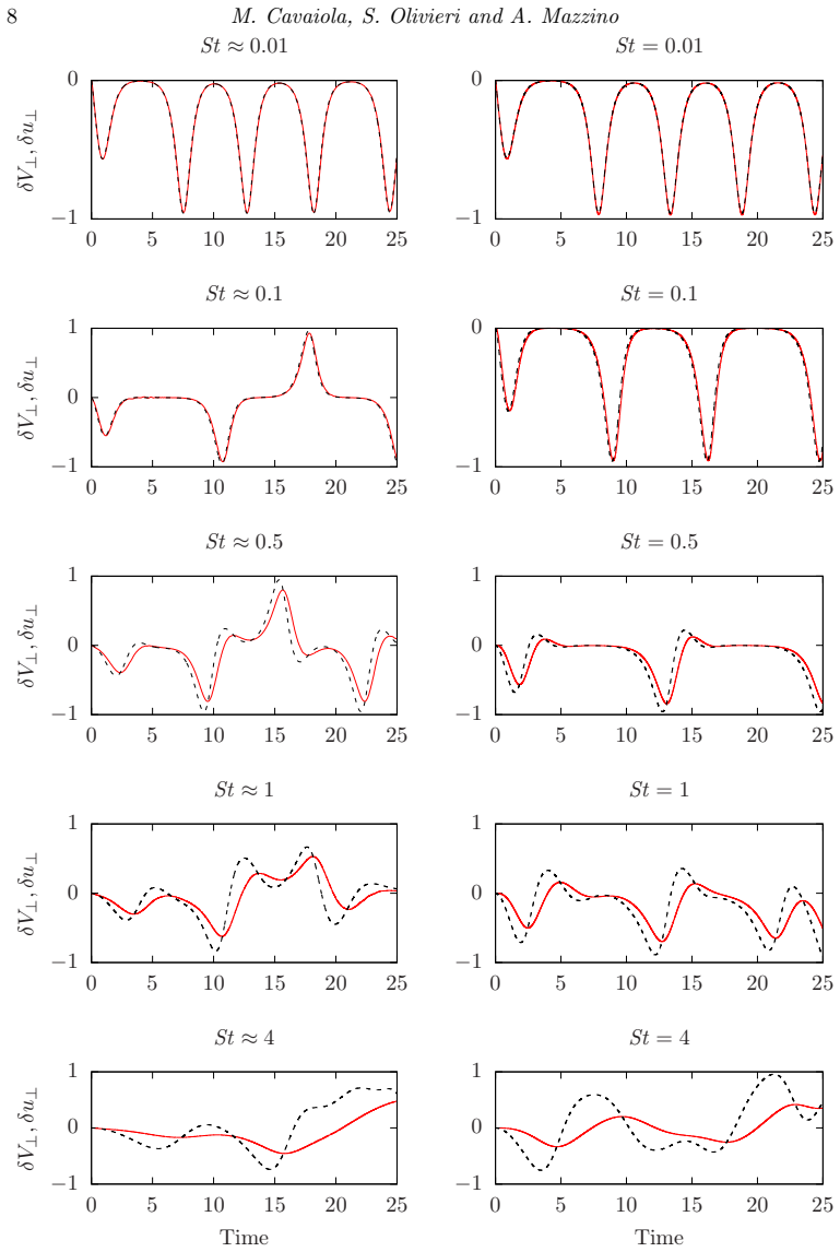
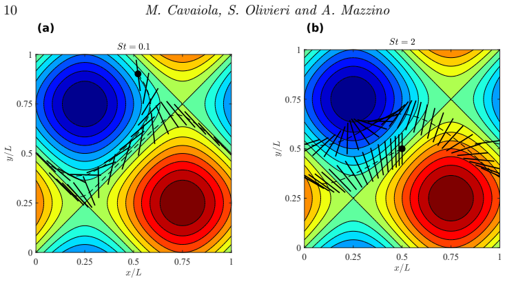
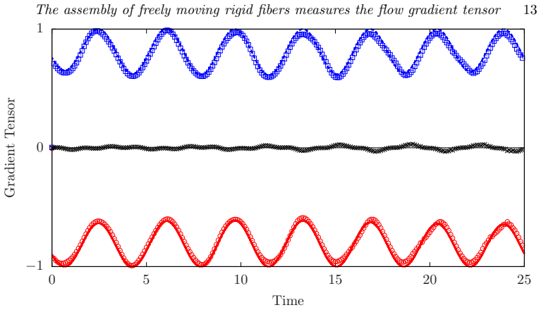
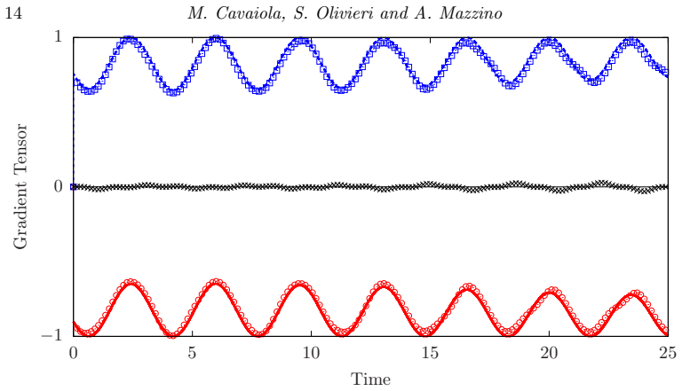
On the paper's own terms, the discovery is that the inextensibility constraint of a rigid fiber, which corrupts single-point velocity measurements, leaves the normal projection of the end-to-end velocity difference clean: $\delta V_\perp = (\mathbf V_B - \mathbf V_A)\cdot \hat{\mathbf r}_\perp$ tracks $\delta u_\perp$, the corresponding unperturbed fluid velocity difference, with deviations below 1% when the rotational Stokes number is $\lesssim 0.1$. For a fiber short compared with the flow's variation scale, $\delta u_\perp$ is well approximated by the tangential-normal projection of the gradient, $D = \partial_j u_i\, \hat r_j\, \hat r_{\perp i}$. With $N_f$ fibers of distinct orientations, equating each measured $\delta V_\perp$ to $D$ yields a linear system (three equations in two-dimensional incompressible flow, eight in three-dimensional flow) whose unknowns are the independent components of $\partial_j u_i$; solving it at each time step reconstructs the gradient tensor. The paper verifies the reconstruction in a steady two-dimensional cellular flow, a steady three-dimensional cellular flow, and a time-periodic two-dimensional flow with chaotic trajectories, using both a fully coupled immersed-boundary simulation and a passive slender-body model.
Load-bearing premise
The whole reconstruction rests on the assumption that a sufficiently light rigid fiber, pulled by the flow, has its two ends move apart in the direction normal to the fiber at the same rate the fluid would, even though the fiber cannot stretch; the paper relies on this $\delta V_\perp \approx \delta u_\perp$ equality without deriving it analytically.
Editorial extensions
If this is right
- A three-fiber assembly yields the full two-dimensional incompressible velocity gradient tensor at every tracked time; an eight-fiber assembly covers three dimensions.
- At rotational Stokes numbers at or below 0.1, the reconstructed gradients match the unperturbed flow to about 1% in the tested steady and time-periodic cellular flows.
- Accuracy degrades as fiber inertia grows, with deviations reaching tens of percent by Stokes numbers of order 0.5–1 and above, so the method has an intrinsic low-inertia operating range.
- The measurement is local and passive, so the same tracked fibers can deliver vorticity, strain rate, and dissipation estimates without resolving the flow at the fiber scale.
- The equality holds for both a fully coupled fiber (including feedback to the flow) and a passive one-way coupled fiber, meaning the hydrodynamic coupling can be neglected in the low-Stokes regime.
Reading between the lines
- If the normal-projection equality persists in turbulence at small Stokes number, a single fiber sampled over many orientations could accumulate gradient information over time, potentially reducing the number of fibers needed below the static assembly count.
- Using two independent normal projections per fiber in three dimensions would overdetermine the system and could improve robustness to measurement noise, an option the paper does not explore.
- The same end-point velocity-difference principle could measure two-point structure functions directly, without first reconstructing the gradient, by comparing normal-projected increments for fibers of different lengths.
- A laboratory test with millimetric rigid fibers in a water tunnel, checked against PIV-derived gradients, would settle whether the 1% numerical accuracy survives optical tracking noise and finite-size effects; the paper stops short of such an experiment.
Signed reviews
Editorial analysis
A structured set of objections, weighed in public.
Referee Report
Summary. The paper proposes a method, termed 'Fiber Tracking Velocimetry', by which the full velocity gradient tensor of a fluid flow can be reconstructed from the Lagrangian tracking of a rigid-fiber assembly. The method relies on the transverse velocity difference between the two ends of each fiber, projected on the direction normal to the fiber, and equates this measured quantity to the corresponding projection of the unperturbed fluid velocity difference. The authors test this idea in two-dimensional steady BC flow, two-dimensional time-periodic oscillating flow, and three-dimensional ABC flow, using both a fully-resolved immersed-boundary (active) model and a passive slender-body model. They report that for Stokes numbers St <= 0.1 the transverse velocity difference measured by the fiber matches the fluid quantity with less than 1% normalized RMS deviation, and that in the two-dimensional cases an assembly of three fibers reconstructs the gradient components with roughly 1% error. The paper claims this capability extends to three dimensions with an eight-fiber assembly.
Significance. If the central equality between fiber-transverse velocity increments and fluid-transverse velocity increments holds, the paper introduces a conceptually novel measurement paradigm that could provide multi-point flow statistics in laboratory and field settings, complementing PIV/PTV. The numerical methodology is thorough: both active and passive fiber models are used, resolution convergence is assessed, and quantitative error metrics are reported for a range of Stokes numbers. The two-dimensional reconstruction results are internally consistent and the comparison between active and passive models for small St is a useful practical insight. However, the theoretical basis of the key equality is heuristic, and, as detailed below, the three-dimensional claim is not supported by the presented evidence and appears mathematically impossible with the chosen projection.
major comments (2)
- [§3.2 and §3.3] The three-dimensional claim of reconstructing the whole gradient tensor is unsupported and, with the stated projection r̂⊥=(r̂2,−r̂1,0), mathematically impossible. In 3D, the quantity D=∂jui r̂j r̂⊥i involves only the six components in the first two rows of ∂jui, namely ∂x u, ∂y u, ∂z u, ∂x v, ∂y v, ∂z v; the components ∂x w and ∂y w never appear, and incompressibility only relates ∂z w to −(∂x u+∂y v). Consequently, the linear system (3.9) formed from any number of fibers using this projection has rank at most six (actually six independent columns, with possible additional degeneracies from fiber alignment), so the full 3×3 gradient cannot be recovered. The paper does not simulate an eight-fiber 3D assembly; §3.2 only demonstrates single-fiber agreement of δV⊥ vs δu⊥ in ABC flow, which does not establish observability of the missing components. Please either restrict the central claim and title to two dimensions, or provide a projection/geometry in 3D that actually probes the third row of the gradient.
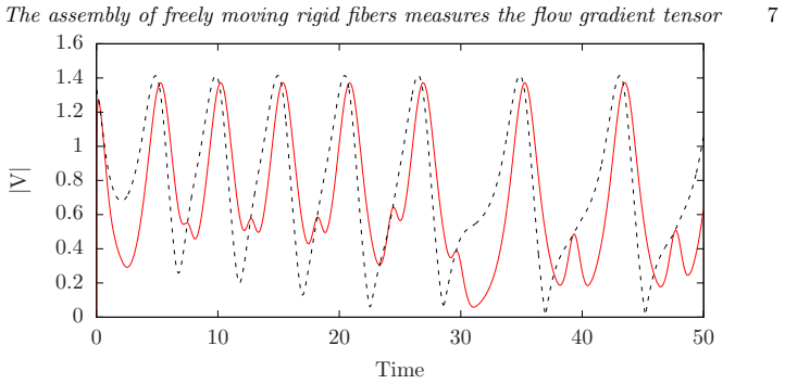
- [§3.1.2, Eqs. (3.4)–(3.6)] The load-bearing premise δV⊥≈δu⊥ is asserted with the heuristic that the inextensibility constraint is 'washed out' in the normal direction, and it is validated numerically for specific flows and parameters, but it is not derived. Since Eq. (3.9) inherits this premise, the reconstruction's validity outside the tested cases is an unquantified risk. Please provide a derivation from the fiber equation of motion (e.g., from Eq. (2.1) with the limits St→0 and c/L→0) showing that δV⊥−δu⊥ scales as O(St) plus O((c/L)^2) or similar, with explicit error bounds. This would also clarify why the agreement degrades as observed in Figures 4 and 6.
minor comments (5)
- [Eq. (3.9)] The linear system is presented as a list of equations; please write it explicitly in matrix form Ax=b and state whether the solution is obtained by direct inversion or least squares, especially for the overdetermined cases mentioned in §3.3.
- [Figure 4 caption] There is a typographical error in the caption: 'St /greaterorequalslant1' should read 'St ≥ 1'.
- [§3.2] The statement 'results do not change for a different choice of r̂⊥' in three dimensions is made without quantitative support. Since the choice of projection is crucial to the method, please show at least one comparison for an alternative normal vector, or clarify that this claim refers only to the plotted single-fiber time series.
- [§3.3] The symbol L is used for the domain size in §2 but is not explicitly defined in the assembly section; please define it at first use when referring to c/L.
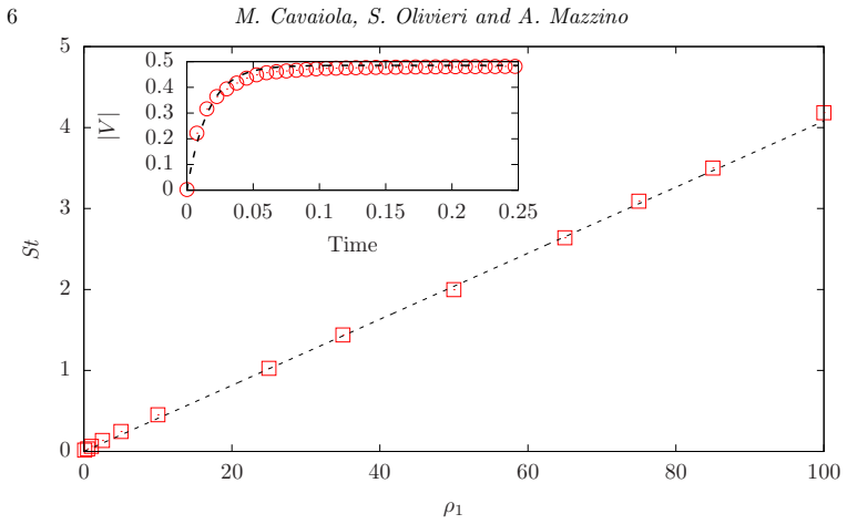
- [§3.3] The claim that the assembly Stokes time equals that of a single fiber is based on the exponential fitting procedure of §3.1.1; please report the fitted values and their uncertainty for the assembly case.
Circularity Check
No significant circularity: the gradient reconstruction is benchmarked against analytic flows, with only a calibration parameter and motivational self-citations.
full rationale
The paper's derivation chain is not circular. The central claim is a numerical validation: fiber end velocity differences projected normal to the fiber, δV⊥, are compared with the unperturbed analytic flow's δu⊥ in BC, ABC, and oscillating cellular flows (Figures 4 and 6), and the gradient reconstruction in §3.3 solves the linear system (3.9) whose coefficients r̂_j r̂⊥_i and data δV⊥ come from tracking the fibers. The reconstructed ∂jui is then compared against the analytic flow gradients (Figures 8–10), which is an external benchmark rather than a fitted output. The only fitted quantity, the rotational Stokes time α from the exponential fit (3.3) in §3.1.1, calibrates the passive model's Stokes time and characterizes inertia; it is not one of the target gradient components and does not appear as a predicted quantity in the reconstruction. Self-citations, notably Rosti et al. (2018a, 2019), motivate the fiber-proxy idea but are not used to justify the BC/ABC/oscillating-flow checks, which are self-contained against analytic expressions. The heuristic assumption in §3.1.2 that δV⊥ ≈ δu⊥ is an unproved modeling ansatz, but it is tested rather than derived from or identified with the target result; a heuristic assumption is a correctness risk, not circularity. The concern that the chosen r̂⊥ makes the full 3D gradient unobservable is likewise an evidence/correctness issue for the 3D claim, not a case of the reconstruction reducing to its own inputs. Score 1 reflects only the presence of non-load-bearing self-citations and the calibration step, without any circular reduction.
Assumptions & free parameters
free parameters (2)
- Rotational Stokes time scaling α =
α ≈ 0.04 (St = α ρ1)
- Fiber centroid separation in assembly =
Δs (the Lagrangian mesh spacing)
assumptions (4)
- domain assumption Fiber dynamics follows the Euler-Bernoulli beam equation (Eq. 2.1) with local drag forcing (Eq. 2.7).
- domain assumption The test flows (BC, ABC, and time-periodic flow) are prescribed solutions of the incompressible flow equations (Eqs. 3.1, 3.7, 3.8).
- ad hoc to paper For small Stokes number, the normal projection of the fiber end-to-end velocity difference equals the normal projection of the undisturbed fluid velocity difference (δV⊥ ≈ δu⊥).
- domain assumption The fiber length is small enough that the two-point velocity difference can be replaced by the local velocity gradient at the fiber center (Eq. 3.6).
Cite this review
Pith. "Pith review of The assembly of freely moving rigid fibers measures the flow gradient tensor." pith.science (2026). https://pith.science/paper/VWUCXTBW
@misc{pith2026190804072,
  author       = {Pith},
  title        = {Pith review of: The assembly of freely moving rigid fibers measures the flow gradient tensor},
  year         = {2026},
  howpublished = {\url{https://pith.science/paper/VWUCXTBW}},
  note         = {Machine review of arXiv:1908.04072}
}
read the original abstract
The motion of an assembly of rigid fibers is investigated for different classes of closed streamline flows, steady or time dependent, two dimensional or three dimensional. In our study, the dynamics of the fiber assembly is fully-coupled to the flow field by means of a state-of-the-art immersed boundary method. We show that, for sufficiently small Stokes times of the assembly, the whole flow gradient tensor can be accurately reconstructed by simply tracking the fiber assembly and measuring suitable fiber velocity differences evaluated at the fiber ends. Our results strongly suggest the possibility of using rigid fibers (or assemblies of them) to perform multi-point flow measures, either in laboratory or in field: future experiments are therefore mandatory to inquire the feasibility of a new `Fiber Tracking Velocimetry' technique.
Figures

Figures from the paper (8 more)


Reference graph
Works this paper leans on
-
[1]
, " * write output.state after.block = add.period write newline
ENTRY address author booktitle chapter edition editor howpublished institution journal key month note number organization pages publisher school series title type volume year eprint label extra.label sort.label short.list INTEGERS output.state before.all mid.sentence after.sentence after.block FUNCTION init.state.consts #0 'before.all := #1 'mid.sentence ...
-
[2]
write newline
" write newline "" before.all 'output.state := FUNCTION n.dashify 't := "" t empty not t #1 #1 substring "-" = t #1 #2 substring "--" = not "--" * t #2 global.max substring 't := t #1 #1 substring "-" = "-" * t #2 global.max substring 't := while if t #1 #1 substring * t #2 global.max substring 't := if while FUNCTION word.in bbl.in capitalize " " * FUNCT...
-
[3]
Adrian, R. J. 1991 Particle-imaging techniques for experimental fluid mechanics . Annu. Rev. Fluid Mech. 23 (1), 261--304
work page 1991
-
[4]
Allende, S. , Henry, C. & Bec, J. 2018 Stretching and buckling of small elastic fibers in turbulence . Phys. Rev. Lett. 121 , 154501
work page 2018
-
[5]
Bagheri, S. , Mazzino, A. & Bottaro, A. 2012 Spontaneous symmetry breaking of a hinged flapping filament generates lift . Phys. Rev. Lett. 109 , 154502
work page 2012
-
[6]
Bakhuis, D. , Mathai, V. , Verschoof, R. A. , Ezeta, R. , Lohse, D. , Huisman, S. G. & Sun, C. 2019 Statistics of rigid fibers in strongly sheared turbulence . Phys. Rev. Fluids 4 , 072301
work page 2019
-
[7]
Banaei, A. A. , Rosti, M. E. & Brandt, L. 2020 Numerical study of filament suspensions at finite inertia . J. Fluid Mech. 882 , A5
2020
-
[8]
Bec, J. , Biferale, L. , Boffetta, G. , Celani, A. , Cencini, M. , Lanotte, A. , Musacchio, S. & Toschi, F. 2006 Acceleration statistics of heavy particles in turbulence . J. Fluid Mech. 550 , 349–358
work page 2006
Show all 49 references
-
[9]
, Biferale, L
Bec, J. , Biferale, L. , Cencini, M. , Lanotte, A. , Musacchio, S. & Toschi, F. 2007 Heavy particle concentration in turbulence at dissipative and inertial scales . Phys. Rev. Lett. 98 , 084502
2007
-
[10]
, Crisanti, A
Biferale, L. , Crisanti, A. , Vergassola, M. & Vulpiani, A. 1995 Eddy diffusivities in scalar transport . Phys. Fluids 7 (11), 2725--2734
1995
-
[11]
, Bouchet, G
Bounoua, S. , Bouchet, G. & Verhille, G. 2018 Tumbling of inertial fibers in turbulence . Phys. Rev. Lett. 121 , 124502
2018
-
[12]
2019 Fiber Tracking Velocimetry
Brizzolara, S. 2019 Fiber Tracking Velocimetry . Master Thesis, U niversity of Genova (Italy), url: https://www.dropbox.com/s/fegtpb03n1uahjm/FTV.pdf?dl=0
2019
-
[13]
Butler, J. E. & Snook, B. 2018 Microstructural dynamics and rheology of suspensions of rigid fibers . Annu. Rev. Fluid Mech. 50 (1), 299--318 , arXiv:arXiv: https://doi.org/10.1146/annurev-fluid-122316-045144
2018 doi
-
[14]
Cartwright, J. H. E. , Feudel, U. , K \'a rolyi, G. , de Moura, A. , Piro, O. & T \'e l, T. 2010 Dynamics of Finite-Size Particles in Chaotic Fluid Flows\/ , pp. 51--87 . Berlin, Heidelberg: Springer Berlin Heidelberg
2010
-
[15]
, Crisanti, A
Castiglione, P. , Crisanti, A. , Mazzino, A. , Vergassola, M. & Vulpiani, A. 1998 Resonant enhanced diffusion in time-dependent flow . J. Phys. A: Math. Gen. 31 (35), 7197--7210
1998
-
[16]
& Uhlmann, M
Chouippe, A. & Uhlmann, M. 2015 Forcing homogeneous turbulence in direct numerical simulation of particulate flow with interface resolution and gravity . Phys. Fluids 27 (12), 123301 , arXiv:arXiv: https://doi.org/10.1063/1.4936274
2015 doi
-
[17]
Cox, R. G. 1970 The motion of long slender bodies in a viscous fluid part 1. general theory . Journal of Fluid Mechanics 44 (4), 791–810
1970
-
[18]
, Amberg, G
Do-Quang, M. , Amberg, G. , Brethouwer, G. & Johansson, A. V. 2014 Simulation of finite-size fibers in turbulent channel flows . Phys. Rev. E 89 , 013006
2014
-
[19]
, Frisch, U
Dombre, T. , Frisch, U. , Greene, J. M. , H\'enon, M. , Mehr, A. & Soward, A. M. 1986 Chaotic streamlines in the ABC flows . J. Fluid Mech. 167 , 353–391
1986
-
[20]
& Fessler, J.R
Eaton, J.K. & Fessler, J.R. 1994 Preferential concentration of particles by turbulence . Int. J. Multiph. Flow 20 , 169 -- 209
1994
-
[21]
, Sheikh, M
Gustavsson, K. , Sheikh, M. Z. , Lopez, D. , Naso, A. , Pumir, A. & Mehlig, B. 2019 Effect of fluid inertia on the orientation of a small prolate spheroid settling in turbulence . New J. Phys. 21 (8), 083008
2019
-
[22]
, Krellenstein, M
Hejazi, B. , Krellenstein, M. & Voth, G. A. 2019 Using deformable particles for single-particle measurements of velocity gradient tensors . Exp. Fluids 60 (10), 153
2019
-
[23]
, Holzner, M
Hoyer, K. , Holzner, M. , L \"u thi, B. , Guala, M. , Liberzon, A. & Kinzelbach, W. 2005 3D scanning particle tracking velocimetry . Exp. Fluids 39 (5), 923
2005
-
[24]
, Shin, S
Huang, W.-X. , Shin, S. J. & Sung, H. J. 2007 Simulation of flexible filaments in a uniform flow by the immersed boundary method . J. Comput. Phys. 226 (2), 2206 -- 2228
2007
-
[25]
Proceedings of the Royal Society of London
Jeffery, George Barker 1922 The motion of ellipsoidal particles immersed in a viscous fluid . Proceedings of the Royal Society of London. Series A, Containing papers of a mathematical and physical character 102 (715), 161--179
1922
-
[26]
, Holzner, M
Krug, D. , Holzner, M. , L \"u thi, B. , Wolf, M. , Tsinober, A. & Kinzelbach, W. 2014 A combined scanning PTV / LIF technique to simultaneously measure the full velocity gradient tensor and the 3D density field . Meas. Sci. Technol. 25 (6), 065301
2014
-
[27]
, Sabban, L
Kuperman, S. , Sabban, L. & van Hout, . 2019 Inertial effects on the dynamics of rigid heavy fibers in isotropic turbulence . Phys. Rev. Fluids 4 , 064301
2019
-
[28]
, Brosse, N
L \=a cis, U. , Brosse, N. , Ingremeau, F. , Mazzino, A. , Lundell, F. , Kellay, H. & Bagheri, S. 2014 Passive appendages generate drift through symmetry breaking . Nat. Commun. 5 , 5310
2014
-
[29]
, Olivieri, S
L \=a cis, U. , Olivieri, S. , Mazzino, A. & Bagheri, S. 2017 Passive control of a falling sphere by elliptic-shaped appendages . Phys. Rev. Fluids 2 , 033901
2017
-
[30]
Lawson, J. M. & Dawson, J. R. 2014 A scanning PIV method for fine-scale turbulence measurements . Exp. Fluids 55 (12), 1857
2014
-
[31]
, Fantoni, M
Marchioli, C. , Fantoni, M. & Soldati, A. 2010 Orientation, distribution, and deposition of elongated, inertial fibers in turbulent channel flow . Phys. Fluids 22 (3), 033301
2010
-
[32]
, Zhao, L
Marchioli, C. , Zhao, L. & Andersson, H. I. 2016 On the relative rotational motion between rigid fibers and fluid in turbulent channel flow . Phys. Fluids 28 (1), 013301
2016
-
[33]
, Kramel, S
Ni, R. , Kramel, S. , Ouellette, N. T. & Voth, G. A. 2015 Measurements of the coupling between the tumbling of rods and the velocity gradient tensor in turbulence . J. Fluid Mech. 766 , 202–225
2015
-
[34]
, Calzavarini, E
Parsa, S. , Calzavarini, E. , Toschi, F. & Voth, G. A. 2012 Rotation rate of rods in turbulent fluid flow . Phys. Rev. Lett. 109 , 134501
2012
-
[35]
, Shelley, M
Quennouz, N. , Shelley, M. , Du Roure, O. & Lindner, A. 2015 Transport and buckling dynamics of an elastic fibre in a viscous cellular flow . J. Fluid Mech. 769 , 387--402
2015
-
[36]
Roma, A. M. , Peskin, C. S. & Berger, M. J. 1999 An adaptive version of the immersed boundary method . J. Comput. Phys. 153 (2), 509 -- 534
1999
-
[37]
Rosti, M. E. , Banaei, A. A. , Brandt, L. & Mazzino, A. 2018 a\/ Flexible fiber reveals the two-point statistical properties of turbulence . Phys. Rev. Lett. 121 , 044501
2018
-
[38]
Rosti, M. E. & Brandt, L. 2017 Numerical simulation of turbulent channel flow over a viscous hyper-elastic wall . J. Fluid Mech. 830 , 708--735
2017
-
[39]
Rosti, M. E. , Izbassarov, D. , Tammisola, O. , Hormozi, S. & Brandt, L. 2018 b\/ Turbulent channel flow of an elastoviscoplastic fluid . J. Fluid Mech. 853 , 488--514
2018
-
[40]
Rosti, M. E. , Olivieri, S. , Banaei, A. A. , Brandt, L. & Mazzino, A. 2019 Flowing fibers as a proxy of turbulence statistics . Meccanica
2019
-
[41]
, Lindner, A
du Roure, O. , Lindner, A. , Nazockdast, E. N. & Shelley, M. J. 2019 Dynamics of flexible fibers in viscous flows and fluids . Annu. Rev. Fluid Mech. 51 (1), 539--572
2019
-
[42]
, Cohen, A
Sabban, L. , Cohen, A. & van Hout, R. 2017 Temporally resolved measurements of heavy, rigid fibre translation and rotation in nearly homogeneous isotropic turbulence . J. Fluid Mech. 814 , 42–68
2017
-
[43]
, Gesemann, S
Schanz, D. , Gesemann, S. & Schr \"o der, A. 2016 Shake-the-box: Lagrangian particle tracking at high particle image densities . Exp. Fluids 57 (5), 70
2016
-
[44]
, Zade, S
Shahmardi, A. , Zade, S. , Ardekani, M. N. , Poole, R. J. , Lundell, F. , Rosti, M. E. & Brandt, L. 2019 Turbulent duct flow with polymers . J. Fluid Mech. 859 , 1057--1083
2019
-
[45]
Shelley, M. J. & Zhang, J. 2011 Flapping and bending bodies interacting with fluid flows . Annu. Rev. Fluid Mech. 43 , 449--465
2011
-
[46]
2004 Simulating the dynamics and interactions of flexible fibers in stokes flows
Tornberg, Anna-Karin & Shelley, Michael J. 2004 Simulating the dynamics and interactions of flexible fibers in stokes flows . Journal of Computational Physics 196 (1), 8 -- 40
2004
-
[47]
Voth, G. A. & Soldati, A. 2017 Anisotropic particles in turbulence . Annu. Rev. Fluid Mech. 49 (1), 249--276
2017
-
[48]
, Quennouz, N
Wandersman, E. , Quennouz, N. , Fermigier, M. , Lindner, A. & du Roure, O. 2010 Buckled in translation . Soft Matter 6 , 5715--5719
2010
-
[49]
& Shelley, M
Young, Y.N. & Shelley, M. J. 2007 Stretch-coil transition and transport of fibers in cellular flows . Phys. Rev. Lett. 99 , 058303
2007
Reviewed August 14, 2026 · model on record in the stance chip above.
Discussion (0). Continue with ORCID to comment.