REVIEW 4 major objections 4 minor 32 references
Solving high-dimensional nonlinear filtering problems using a tensor train decomposition method
T0 review · 4 major / 4 minor · reviewed 2026-08-14 · deepseek-v4-flash
Pith's one-line read Quantized tensor trains solve 3D nonlinear filtering in seconds
desk verdict A promising QTT-based filter for 3D problems whose central complexity claim does not survive its own Table 5. read the letter →
The pith
A machine-rendered reading of the paper's core claim, the machinery that carries it, and where it could break.
The reading
What carries the argument
The central object is the quantized tensor train (QTT) decomposition: a $d$-dimensional tensor is written as a product of small cores $G_1(i_1)\cdots G_d(i_d)$ with TT-ranks $r_k$, and each spatial dimension is reshaped into virtual binary dimensions so storage drops to $O(d\log_2(N) r^2)$. The method's engine is the exponential transformation $\sigma(x,t)=\exp(h^T(x,t)S^{-1}(t)y_t)u(x,t)$, which converts the stochastic DMZ equation into a deterministic FKE, plus the offline assembly of the operator $A=\frac12\Delta_d-C_d-\frac12 Q_d$ in QTT format and its power $(\tau A+I)^{\Delta T/\tau}$. The QTT rank of the discrete Laplacian is bounded by 4, the convection operator's rank by $5dr$ when the drift functions have rank $r$, and TT-SVD rounding controls the ranks of everything else; these bounds are what make the online operations — Hadamard products and matrix-vector products — fast.
What would settle it
Run a filtering problem whose conditional density becomes more complex over time — for example, a bimodal drift that splits the density into well-separated peaks, or a cubic sensor in four dimensions — and record the effective QTT rank at each observation time. If the rank exceeds the assumed constant bound and keeps growing, the stated online complexity and convergence guarantee will not hold.
Extended reading notes
Core claim
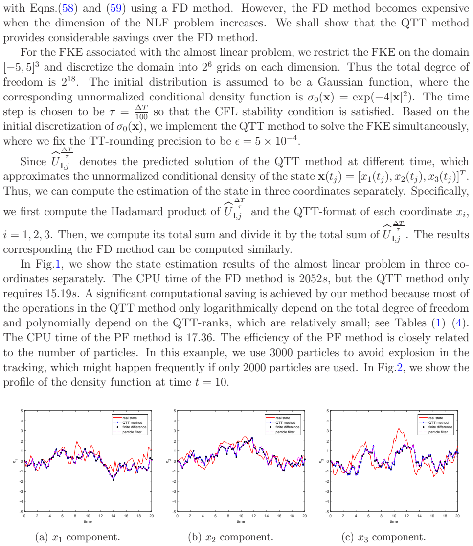
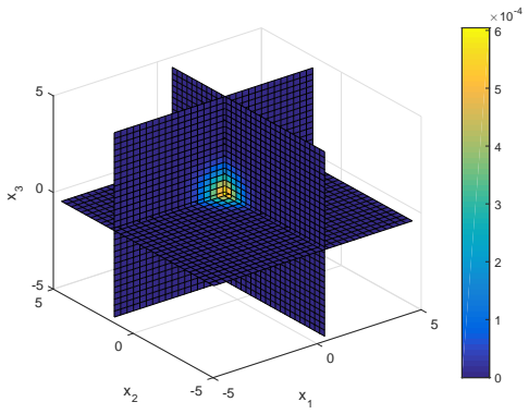
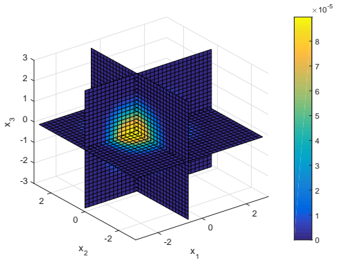
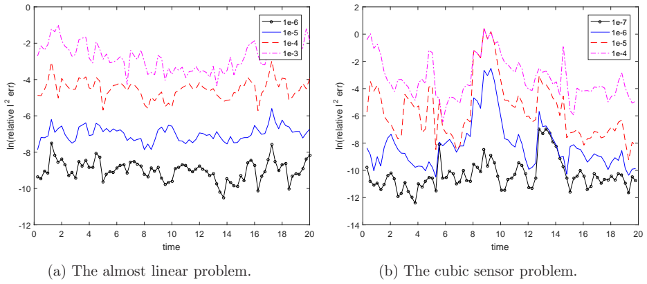
On the paper's own terms, the central discovery is that the forward Kolmogorov equation (FKE) — a parabolic PDE for the unnormalized conditional density — admits low-rank quantized tensor train representations over the filtering horizon, so the whole filtering loop can be run in compressed form. Starting from the pathwise robust DMZ equation (the stochastic PDE for the unnormalized conditional density), the paper freezes each observation interval, solves the FKE with a finite-difference operator assembled in QTT format, and assimilates new observations through the exponential transformation. Theorem 5.7 bounds the $L^1$ error between the QTT-recovered density and the DMZ solution by three contributions: the time-frozen approximation of the observation path, the finite-difference discretization error $O(\tau+h^2)$, and the QTT rounding errors. Numerically, the method matches finite-difference estimates on two 3D examples (mean-square errors $0.007$ and $0.023$) while cutting the per-run CPU time from $2052$ s and $4079$ s to about $15$ s and $17$ s.
Load-bearing premise
The method works only if the compressed representation of the density stays small over the entire filtering window; the paper assumes exactly this (Proposition 4.3) and checks it numerically on only two three-dimensional examples. If the compression size grows with time or dimension, the promised speed-up and the error bound both collapse.
Editorial extensions
If this is right
- If the ranks stay bounded, the online per-interval cost is $O(d\log_2(N) r^6)$, so refining the spatial grid makes the solver only logarithmically more expensive.
- The offline/online split means the same low-rank propagator can be reused for every observation path of a given system, making repeated or long-horizon filtering much cheaper after a one-time setup.
- Theorem 5.7 gives explicit error control: reduce $N_t$ for the path-frozen error, $\tau$ and $h$ for the finite-difference error, and the TT-rounding precisions for the QTT error.
- In the two 3D examples, the method matches the finite-difference density estimates while reducing CPU time from 2052 s and 4079 s to about 15 s and 17 s.
Reading between the lines
- A natural stress test, not performed in the paper, is a time-dependent drift or observation function: the paper itself notes the low-rank structure may shift over time, so an adaptive or dynamic low-rank update would be needed.
- The offline phase must build low-rank QTT tensors from full discretized operators; the paper reports this cost is modest for the 3D tests, but for much larger $d$ or $N$ the offline construction could become the bottleneck unless cross-approximation is used.
- Assumption 4 requires the observation term $|2h^T y_t|$ to be bounded by a constant, but real observations driven by Brownian motion are not bounded; a fully rigorous guarantee would need a truncation of observations or a probabilistic bound on the exceptional paths.
- If the small-rank conjecture survives in $d>3$, the $O(N d r^2)$ cost of assimilating the exponential observation factor becomes the main bottleneck, so the scaling in very high dimension deserves direct measurement.
Signed reviews
Editorial analysis
A structured set of objections, weighed in public.
Referee Report
Summary. The paper proposes a tensor-train (QTT) method for solving the forward Kolmogorov equation (FKE) that arises in nonlinear filtering, with an offline stage that precomputes low-rank QTT representations of the discretized PDE operators and propagator, and an online stage that assimilates observations through an exponential (Hadamard) update and propagates the density in QTT format. A convergence theorem (Theorem 5.7) is stated that combines the observation-time splitting error, the finite-difference discretization error, and the QTT rounding errors. Numerical experiments on two 3D filtering problems compare the method against finite differences and particle filters, reporting large speedups at moderate resolution and small mean-square errors relative to the FD reference.
Significance. If the assumed low-rank structure persists, the method is a promising route toward real-time nonlinear filtering: the paper gives explicit convergence analysis, identifies the three sources of error separately, and demonstrates on two 3D examples that the FKE density has low effective QTT ranks, yielding speedups of two orders of magnitude over finite differences. The numerical comparison is honest in reporting averaged MSEs over 100 paths and in showing convergence with respect to the TT-rounding precision. However, the high-dimensional and real-time claims go beyond what is demonstrated: only d=3 is tested, and the complexity analysis contains a load-bearing gap that the paper's own timing data contradicts.
major comments (4)
- [Section 4.3, Proposition 4.3 and Table 5] The claimed O(N d r^2) cost for constructing exp[h^T(x,t_j)(y_{t_j}-y_{t_{j-1}})] in QTT format is contradicted by the paper's own timing data. The proof says this is obtained 'from a full multidimensional array' via Theorem 2.1 of [25], but a full array has N^d entries; the cited theorem does not justify a construction that avoids materializing the full array for a general nonlinear h(x)\cdot y_t. In Table 5, doubling N from 64 to 128 increases tEXP from 5.20 s to 46.28 s (a factor of 8.9), while the averaged QTT rank grows only from 8.78 to 8.89; this scaling is close to O(N^d), not O(N d r^2). Since this step is repeated at every observation time, the online complexity stated in Proposition 4.3 and the associated real-time claim are not supported.
- [Section 5.1, Assumption (Asm.4) and Lemma 5.4] The convergence theorem requires |2h^T y_t| \le c2 on the observation times, but for the SDE model (2) the observation process y_t is not bounded. Even with h bounded on the numerical domain, h^T y_t is unbounded along a Brownian path; for a fixed path the maximum is finite, but the resulting constant c2 is path-dependent and typically grows with the number of observation times, and the paper does not quantify it. The constant c2 controls the factor e^{c2} in Eq. (42) and enters the final bounds (36) and (53). The numerical experiments do not indicate that the simulated observation paths are truncated or that Asm.4 is verified, so the convergence statement as formulated does not cover the stochastic model actually simulated in Section 6.
- [Section 5.3, Lemma 5.5 and Theorem 5.7] The QTT contribution to the error is controlled by powers c7^{Nt}, with c7 = (1+ǫ1)(1+ǫ2)c6 e^{c2} defined after Eq. (49). The paper does not show that c7 < 1, and for a stable explicit scheme with c6 potentially larger than 1 this will generally not be the case. Consequently, the term ǫ1 c7^{Nt} in Eq. (46) and the analogous terms in (53) grow exponentially in the number of observations, so the displayed bound does not establish an error of order O(Nt^{-α} + τ + h^2 + ǫ1 + ǫ2) uniformly in Nt. As stated, the convergence theorem is therefore not proven by the given estimates unless the authors add a mechanism (such as explicit conditions guaranteeing c7 < 1 or a choice of ǫ1, ǫ2 that compensates the exponential growth).
- [Abstract, Section 7, and Section 6] The paper claims in the abstract and conclusions that it solves 'high-dimensional' NLF problems in a real-time manner, but all numerical experiments are for d=3 (Examples 1 and 2 in Section 6.2). The central assumption of bounded QTT ranks (Proposition 4.3) is verified only for these 3D problems, as shown in Tables 1-4; no evidence is provided for d>3, and Section 7 itself defers d>3 to future work. The high-dimensional claim in the title and abstract is therefore an overstatement of the demonstrated results.
minor comments (4)
- [Abstract] The word 'roblem' in 'NLF roblem' is a typo and should be corrected to 'problem'.
- [Section 6.3, Table 5] The table should specify whether tFKE and tEXP are total costs over the whole simulation or per observation interval; the text says the FD method at N=2^7 would cost about 13 hours, but without a per-step breakdown the real-time claim cannot be checked against the observation interval ΔT=0.05.
- [Section 6.1, Eq. (60)] The definition of the effective QTT-rank r_eff is nonstandard and not derived; the authors should either explain its motivation or report the maximum QTT-rank, which is the quantity that enters the complexity estimates.
- [References] Reference [14] has a typo in the author name: 'Vlanimir A. Kazeev' should be 'Vladimir A. Kazeev'.
Circularity Check
No significant circularity: the QTT solution is compared against independent finite-difference and particle-filter references, and the cited self-results are parameter-free theorems used as background.
full rationale
The paper's derivation chain is standard and non-circular: the DMZ equation is transformed into the pathwise robust DMZ equation using the exponential change of variables from Yau and Yau [30], then into a forward Kolmogorov equation, which is discretized by finite differences and solved in QTT format. The convergence analysis in Theorem 5.7 is a triangle-inequality splitting into three independent error terms: the time-freezing error (Proposition 5.1, cited from [30]), the finite-difference discretization error (Lemma 5.4), and the QTT-rounding error (Lemma 5.5). Each term is proven separately and the cited propositions are external, parameter-free mathematical theorems with stated assumptions that do not include the present paper's numerical results; the fact that [30] shares an author is therefore not load-bearing circularity. The central numerical claim is validated against finite-difference and particle-filter benchmarks, not against a fitted quantity, so there is no 'fitted input called prediction' pattern. The bounded-rank assumption in Proposition 4.3 is an explicit assumption, and the paper verifies slow rank growth numerically in Tables 1-4; this is an empirical check, not a circular definition. Potential concerns about the complexity statement in Proposition 4.3, such as the claim that a full multidimensional array can be converted to QTT format in O(N d r^2) time when the array has N^d entries, or the scaling of tEXP in Table 5 being inconsistent with linear-in-N growth, are correctness and rigor issues rather than circularity: they do not make the derived result equivalent to its input by construction. Overall, no step in the paper's derivation reduces to its own assumptions or to a self-citation chain.
Assumptions & free parameters
assumptions (4)
- domain assumption Pathwise robust DMZ equation is well-posed and equivalent to the FKE under growth conditions on f and h with at most linear growth.
- domain assumption Observation paths satisfy |2 h^T y_t| <= c2 (Asm.4), so the exponential transformation is bounded and the domain truncation is valid.
- ad hoc to paper The QTT-ranks of operators and of the solution remain bounded by a small r throughout the evolution.
- standard math Explicit finite-difference stability conditions h < 1/Cf and tau < (d/h^2 + dLf + d/2 Ch^2)^{-1} hold.
Cite this review
Pith. "Pith review of Solving high-dimensional nonlinear filtering problems using a tensor train decomposition method." pith.science (2026). https://pith.science/paper/W2HQHOWG
@misc{pith2026190804010,
  author       = {Pith},
  title        = {Pith review of: Solving high-dimensional nonlinear filtering problems using a tensor train decomposition method},
  year         = {2026},
  howpublished = {\url{https://pith.science/paper/W2HQHOWG}},
  note         = {Machine review of arXiv:1908.04010}
}
read the original abstract
In this paper, we propose an efficient numerical method to solve high-dimensional nonlinear filtering (NLF) problems. Specifically, we use the tensor train decomposition method to solve the forward Kolmogorov equation (FKE) arising from the NLF problem. Our method consists of offline and online stages. In the offline stage, we use the finite difference method to discretize the partial differential operators involved in the FKE and extract low-dimensional structures in the solution space using the tensor train decomposition method. In addition, we approximate the evolution of the FKE operator using the tensor train decomposition method. In the online stage using the pre-computed low-rank approximation tensors, we can quickly solve the FKE given new observation data. Therefore, we can solve the NLF roblem in a real-time manner. Under some mild assumptions, we provide convergence analysis for the proposed method. Finally, we present numerical results to show the efficiency and accuracy of the proposed method in solving high-dimensional NLF problems.
Figures

Figures from the paper (2 more)
Reference graph
Works this paper leans on
-
[25]
I. V. Oseledets. Approximation of 2 d × 2d matrices using tensor decomposition. SIAM Journal on Matrix Analysis and Applicatoins , 31(4):2130–2145, 2010
work page 2010
-
[30]
Real time solution of the n onlinear filtering problem without memory II
Shing-Tung Yau and Stephen S-T Yau. Real time solution of the n onlinear filtering problem without memory II. SIAM Journal on Control and Optimization , 47(1):163–195, 2008
work page 2008
-
[1]
M. S. Arulampalam, S. Maskell, N. Gordon, and T. Clapp. A tutorial on particle filters for online nonlinear/non-gaussian Bayesian tracking. IEEE Transactions on signal processing, 50(2):174–188, 2002
work page 2002
-
[2]
A. Bain and D. Crisan. Fundamentals of stochastic filtering , volume 3. Springer, 2009
work page 2009
- [3]
-
[4]
A. Bensoussan, R. Glowinski, and A. Rascanu. Approximation of t he Zakai equation by the splitting up method. SIAM Journal on Control and Optimization , 28(6):1420–1431, 1990. 26
work page 1990
- [5]
- [6]
Show all 32 references
-
[7]
S. V. Dolgov, B. N. Khoromskij, and I. V. Oseledets. Fast solutio n of parabolic problems in the tensor train/quantized tensor train format with initial applica tion to the Fokker- Planck equation. SIAM Journal on Scientific Computing , 34(6):A3016–A3038, 2012
2012
-
[8]
T. Duncan. Probability densities for diffusion processes with applic ations to nonlinear filtering theory and detection theory. Technical report, Stanford Univ CA Stanford Elec- tronics Labs, 1967
1967
-
[9]
Fleming and S
W. Fleming and S. Mitter. Optimal control and nonlinear filtering fo r nondegenerate diffusion processes. Stochastics, 8(1):63–77, 1982
1982
-
[10]
Gustafsson, F
F. Gustafsson, F. Gunnarsson, N. Bergman, U. Forssell, J. J ansson, R. Karlsson, and P. J. Nordlund. Particle filters for positioning, navigation, and tracking. IEEE Transactions on signal processing , 50(2):425–437, 2002
2002
-
[11]
Gy¨ ongy and N
I. Gy¨ ongy and N. Krylov. On the splitting-up method and stoch astic partial differential equations. The Annals of Probability , 31(2):564–591, 2003
2003
-
[12]
K. Ito. Approximation of the Zakai equation for nonlinear filter ing. SIAM Journal on Control and Optimization , 34(2):620–634, 1996
1996
-
[13]
Kallianpur
G. Kallianpur. Stochastic filtering theory , volume 13. Springer Science & Business Media, 2013
2013
-
[14]
Kazeev, and Boris N
Vlanimir A. Kazeev, and Boris N. Khoromskij. Low-rank explicit QT T representation of the laplace operator and its inverse. SIAM Journal on Matrix Analysis and Applications , 33(3):724–758, 2012
2012
-
[15]
Khoromskij
Boris N. Khoromskij. O(d log N)-Quantics approximation of N − d tensors in high- dimensional numerical modeling. Constructive Approximation , 34:257–280, 2011
2011
-
[16]
P. E. Kloeden and E. Platen. Numerical solution of Stochastic Differential Equations . Springer-Verlag Berlin, Heidelberg, 1992
1992
-
[17]
Kurtz and J
T. Kurtz and J. Xiong. Particle representations for a class of nonlinear SPDEs . Stochastic Processes and their Applications , 83(1):103–126, 1999
1999
-
[18]
H. Kushner. Approximations to optimal nonlinear filters . IEEE Transactions on Auto- matic Control , 12(5):546–556, 1967. 27
1967
-
[19]
Lototsky, R
S. Lototsky, R. Mikulevicius, and B. L. Rozovskii. Nonlinear filter ing revisited: a spectral approach. SIAM Journal on Control and Optimization , 35(2):435–461, 1997
1997
-
[20]
Luo and Stephen S
X. Luo and Stephen S. T. Yau. Complete real time solution of the general nonlinear fil- tering problem without memory. IEEE Transactions on Automatic Control , 58(10):2563– 2578, 2013
2013
-
[21]
Luo and Stephen S
X. Luo and Stephen S. T. Yau. Hermite spectral method to 1-D forward Kolmogorov equation and its application to nonlinear filtering problems. IEEE Transactions on Au- tomatic Control, 58(10):2495–2507, 2013
2013
-
[22]
Mortensen
R. Mortensen. Optimal control of continuous-time stochast ic systems. Technical report, California Univ Berkeley Electronics Research Lab , 1966
1966
-
[23]
Morton and D
K. Morton and D. Mayers. Numerical solution of partial differen tial equations: an intro- duction. Cambridge University Press , 2005
2005
-
[24]
N. Nagase. Remarks on nonlinear stochastic partial differentia l equations: an application of the splitting-up method. SIAM Journal on Control and Optimization , 33(6):1716–1730, 1995
1995
-
[26]
I. V. Oseledets. Tensor-train decomposition. SIAM Journal on Scientific Computing , 33(5):2295-2317, 2011
2011
-
[27]
I. V. Oseledets and E. E. Tyrtyshnikov. TT-cross approximat ion for multidimensional arrays. Linear Algebra and its Applications , 432:70–88, 2010
2010
-
[28]
Pardouxt
E. Pardouxt. Stochastic partial differential equations and filt ering of diffusion processes. Stochastics, 3:127–167, 1980
1980
-
[29]
Z. Wang, X. Luo, Stephen S.-T. Yau, and Z. Zhang. Proper ort hogonal decomposition method to nonlinear filtering problems in medium-high dimension. to appear in IEEE Transactions on Automatic Control , 2020
2020
-
[31]
M. Zakai. On the optimal filtering of diffusion processes. Probability Theory and Related Fields, 11(3):230–243, 1969
1969
-
[32]
Q. Zhang. Nonlinear filtering and control of a switching diffusion w ith small observation noise. SIAM Journal on Control and Optimization , 36(5):1638–1668, 1998. 28
1998
Reviewed August 14, 2026 · model on record in the stance chip above.
Discussion (0). Continue with ORCID to comment.