Loss-Conditional PINNs for Parametric PDE Families
Pith reviewed 2026-06-28 07:25 UTC · model grok-4.3
The pith
A single PINN can solve entire families of PDEs by taking loss weights or physical coefficients as inputs during training.
A machine-rendered reading of the paper's core claim, the machinery that carries it, and where it could break.
Core claim
LC-PINN extends loss-conditional training to the PDE setting by feeding the conditioning vector directly into the network and sampling it from a prior at each optimization step. This produces a continuous family of solutions indexed by the vector. The construction yields a lambda-invariance property at the conditional optimum. Loss-weight conditioning uses simple concatenation while physical-coefficient conditioning uses FiLM layers, together with a fixed-quadrature L-BFGS finishing step. On the tested parametric PDEs a single trained LC-PINN matches or improves upon retrained per-weight baselines while covering the whole family at amortized cost.
What carries the argument
The loss-conditional PINN that receives the conditioning vector (loss weights or physical coefficient) as an explicit input and is trained by sampling that vector from a prior at every step.
If this is right
- A single trained model can be queried for any conditioning value in the sampled range without further optimization.
- Total training cost scales better than per-instance retraining once more than a few different weight or coefficient values are required.
- The same architecture handles both loss-weight families and physical-coefficient families.
- The method applies without modification to the Helmholtz, Schrödinger, viscous Burgers, and Buckley-Leverett equations.
Where Pith is reading between the lines
- The approach could be tested on conditioning variables beyond weights and coefficients, such as domain shape parameters.
- It occupies a middle position between classical PINNs and data-driven operator learners that require paired solution examples.
- For applications that repeatedly solve similar PDEs with modest parameter variation, the amortized cost may eliminate the need for per-instance hyperparameter tuning.
Load-bearing premise
Random sampling of the conditioning vector from a simple prior at each optimization step produces a network whose outputs remain accurate across the entire sampled range without extra regularization.
What would settle it
Train one LC-PINN on a broad range of loss weights for the viscous Burgers equation, then evaluate PDE residual errors at ten conditioning vectors spread across that range; if the errors are substantially larger than those obtained from separately trained PINNs at the same points, the central claim does not hold.
Figures
read the original abstract
Physics-informed neural networks (PINNs) approximate solutions of ODEs and PDEs by minimising a weighted combination of residual, boundary, initial, and data losses. Their performance is often dominated by the choice of loss weights: a poor weighting can drive training to a degenerate solution in which one physical constraint is satisfied while another is ignored. Existing methods select or adapt a single good set of weights. We take a different view: instead of tuning one weight vector, we explore the entire weight space during training. We introduce LC-PINN, which adapts the loss-conditional training of Dosovitskiy and Djolonga (2020) to the PDE-residual setting: the conditioning vector (either the loss weights or a scalar physical coefficient) is treated as a network input and sampled from a simple prior at every optimisation step. This turns PINN training into learning a continuous family of solutions indexed by that vector, with no solver-generated paired data. LC-PINN thus lies between classical PINNs and operator learning: it stays fully physics-informed but amortises training over a parametric family. Our contribution is not the loss-conditional construction itself, but its extension to PINNs, the unification of the loss-weight and parametric-coefficient regimes under one architecture (concatenation for loss weights, FiLM for coefficients), and a fixed-quadrature L-BFGS finishing protocol that makes the parametric-coefficient regime trainable. We give a lambda-invariance result for the conditional optimum and study LC-PINN on parametric Helmholtz, Schrodinger, viscous Burgers, and Buckley-Leverett equations. A single LC-PINN matches or improves retrained per-weight PINN baselines while parameterising the full family in one model, at a total cost that amortises favourably against per-instance retraining.
Editorial analysis
A structured set of objections, weighed in public.
Referee Report
Summary. The manuscript introduces LC-PINN, which extends loss-conditional training to PINNs by feeding a conditioning vector (loss weights or a physical coefficient) as an additional network input and sampling it from a simple prior at every optimization step. This produces a single model that represents a continuous family of PDE solutions without solver-generated paired data. The paper unifies the loss-weight and parametric-coefficient regimes (via concatenation and FiLM respectively), states a lambda-invariance result for the conditional optimum, introduces a fixed-quadrature L-BFGS finishing protocol, and reports experiments on parametric Helmholtz, Schrödinger, viscous Burgers, and Buckley-Leverett equations in which one LC-PINN matches or improves upon retrained per-instance PINN baselines while amortizing total cost.
Significance. If the empirical claims hold after accounting for training variance, LC-PINN supplies a practical middle ground between classical PINNs and operator-learning methods: it remains fully physics-informed, requires no external paired data, and amortizes training over a parametric family. The lambda-invariance result and the L-BFGS finishing protocol are concrete technical contributions that address trainability in the parametric-coefficient setting.
major comments (2)
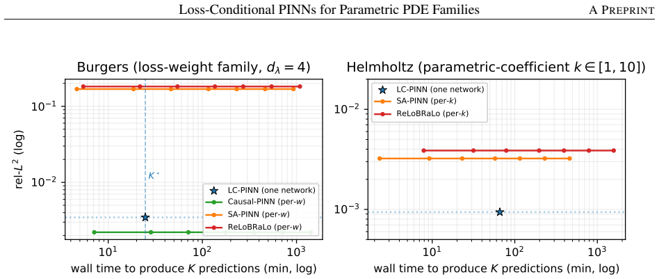
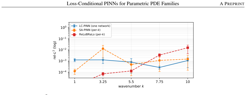
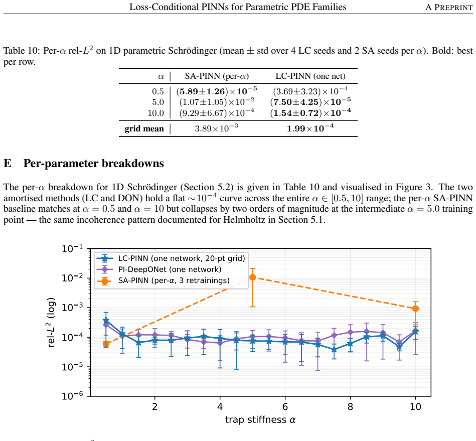
- [Abstract and §4] Abstract and §4 (experiments): the central claim that a single LC-PINN matches or improves retrained per-weight baselines requires explicit per-conditioning error tables (or plots) that compare LC-PINN outputs at fixed conditioning vectors against multiple independent runs of standard PINNs; without such disaggregated metrics it is impossible to verify that joint training with random sampling produces no accuracy trade-offs across the sampled support.
- [§3.1] §3.1 (lambda-invariance result): the invariance is invoked to justify the conditional optimum, yet the manuscript does not state whether the result continues to hold exactly when the conditioning vector is redrawn stochastically at each step or only in expectation; this distinction is load-bearing for the training procedure described in §2.
minor comments (2)
- [§2.2] §2.2: the description of the fixed-quadrature L-BFGS finishing step would benefit from an explicit statement of the quadrature rule and the number of points used, so that the protocol can be reproduced exactly.
- [§4] Figure captions in §4: several plots lack error bars or mention of the number of independent seeds; adding this information would clarify whether reported improvements exceed training variance.
Simulated Author's Rebuttal
We thank the referee for the constructive comments. We address each major point below and will revise the manuscript accordingly.
read point-by-point responses
-
Referee: [Abstract and §4] Abstract and §4 (experiments): the central claim that a single LC-PINN matches or improves retrained per-weight baselines requires explicit per-conditioning error tables (or plots) that compare LC-PINN outputs at fixed conditioning vectors against multiple independent runs of standard PINNs; without such disaggregated metrics it is impossible to verify that joint training with random sampling produces no accuracy trade-offs across the sampled support.
Authors: We agree that disaggregated per-conditioning metrics are required to substantiate the claim. The current experiments report aggregate performance across the family; in the revision we will add tables (and/or supplementary plots) that list, for each fixed conditioning vector, the LC-PINN error together with the mean and standard deviation obtained from multiple independent standard-PINN runs. This will allow direct verification that random-sampling joint training introduces no systematic accuracy trade-offs. revision: yes
-
Referee: [§3.1] §3.1 (lambda-invariance result): the invariance is invoked to justify the conditional optimum, yet the manuscript does not state whether the result continues to hold exactly when the conditioning vector is redrawn stochastically at each step or only in expectation; this distinction is load-bearing for the training procedure described in §2.
Authors: The lambda-invariance result is stated for any fixed conditioning vector. Because the training procedure samples the vector at each step and thereby minimizes the expected loss, the exact conditional optimum for each realized vector remains a stationary point of the expected objective. We will add an explicit sentence in §3.1 clarifying that the invariance holds exactly for each sampled vector (hence the family of conditional optima is recovered in expectation) and will insert a cross-reference in §2. revision: yes
Circularity Check
No significant circularity detected; claims rest on empirical evaluation of a training procedure.
full rationale
The paper describes a training procedure (sampling conditioning vectors from a prior and optimizing a single network) and reports empirical performance on benchmark PDEs against retrained per-instance baselines. No equations, predictions, or optimality results are shown to reduce by construction to fitted inputs, self-citations, or renamed known patterns. The cited lambda-invariance result and external reference to Dosovitskiy and Djolonga (2020) are not load-bearing in a self-referential way. The derivation chain is self-contained against external benchmarks.
Axiom & Free-Parameter Ledger
axioms (1)
- domain assumption Sampling the conditioning vector from a simple prior at each optimization step produces a network that generalizes across the sampled range without collapse to degenerate solutions.
Reference graph
Works this paper leans on
-
[1]
Dosovitskiy and J
A. Dosovitskiy and J. Djolonga. You only train once: loss-conditional training of deep networks. InInternational Conference on Learning Representations (ICLR), 2020
2020
-
[2]
Raissi, P
M. Raissi, P. Perdikaris, and G. E. Karniadakis. Physics-informed neural networks: A deep learning framework for solving forward and inverse problems involving nonlinear partial differential equations.Journal of Computational Physics, 378:686–707, 2019
2019
-
[3]
Z. Li, N. Kovachki, K. Azizzadenesheli, B. Liu, K. Bhattacharya, A. Stuart, and A. Anandkumar. Fourier neural operator for parametric partial differential equations. InInternational Conference on Learning Representations (ICLR), 2021
2021
-
[4]
L. Lu, P. Jin, G. Pang, Z. Zhang, and G. E. Karniadakis. Learning nonlinear operators via deeponet based on the universal approximation theorem of operators.Nature Machine Intelligence, 3(3):218–229, 2021
2021
-
[5]
Arthurs and Andrew P
Christopher J. Arthurs and Andrew P. King. Active training of physics-informed neural networks to aggregate and interpolate parametric solutions to the Navier–Stokes equations.Journal of Computational Physics, 438:110364, 2021
2021
-
[6]
L. McClenny and U. Braga-Neto. Self-adaptive physics-informed neural networks using a soft attention mechanism. arXiv preprint arXiv:2009.04544, 2020
-
[7]
R. Bischof and M. A. Kraus. Multi-objective loss balancing for physics-informed deep learning.arXiv preprint arXiv:2110.09813, 2021
-
[8]
S. Wang, S. Sankaran, and P. Perdikaris. Respecting causality for training physics-informed neural networks. Computer Methods in Applied Mechanics and Engineering, 421:116813, 2024
2024
-
[9]
S. Wang, H. Wang, and P. Perdikaris. Learning the solution operator of parametric partial differential equations with physics-informed deeponets.Science Advances, 7(40):eabi8605, 2021
2021
-
[10]
D. Ha, A. Dai, and Q. V . Le. Hypernetworks. InInternational Conference on Learning Representations (ICLR), 2017
2017
-
[11]
C. Finn, P. Abbeel, and S. Levine. Model-agnostic meta-learning for fast adaptation of deep networks. In International Conference on Machine Learning (ICML), 2017
2017
-
[12]
X. Liu, X. Zhang, W. Peng, W. Zhou, and W. Yao. A novel meta-learning initialization method for physics-informed neural networks.Neural Computing and Applications, 34:14511–14534, 2022
2022
-
[13]
K. Hornik. Approximation capabilities of multilayer feedforward networks.Neural Networks, 4(2):251–257, 1991
1991
-
[14]
A. Pinkus. Approximation theory of the MLP model in neural networks.Acta Numerica, 8:143–195, 1999
1999
-
[15]
Perez, F
E. Perez, F. Strub, H. de Vries, V . Dumoulin, and A. Courville. FiLM: Visual reasoning with a general conditioning layer. InAAAI Conference on Artificial Intelligence (AAAI), 2018. 12 Loss-Conditional PINNs for Parametric PDE FamiliesA PREPRINT A Derivation of the local loss-decay result This appendix provides the details behind Theorem 4.1. The goal is ...
2018
-
[16]
Evaluation grids.Burgers / BL test errors are computed on a 256×101 space–time grid; Helmholtz on a 1024-point spatial grid
cos(πx)g(x;α), which agrees with a centred-difference numerical residual to<5×10 −6 acrossα∈ {0.5,2,5,10}. Evaluation grids.Burgers / BL test errors are computed on a 256×101 space–time grid; Helmholtz on a 1024-point spatial grid. The K-shot averaged LC-PINN prediction is the mean of K forward passes at independent λ samples from pλ; we useK=100for Burge...
discussion (0)
Sign in with ORCID, Apple, or X to comment. Anyone can read and Pith papers without signing in.