REVIEW 4 major objections 6 minor 38 references
On the Incorporation of Box-Constraints for Ensemble Kalman Inversion
T0 review · 4 major / 6 minor · reviewed 2026-08-14 · deepseek-v4-flash
Pith's one-line read A projected ensemble Kalman inversion with variance inflation converges in mean square to the smoothed constrained optimum.
desk verdict The algorithmic idea is plausible and the numerics are informative, but the main convergence theorem has a load-bearing algebraic error and the advertised analysis is not established. read the letter →
The pith
A machine-rendered reading of the paper's core claim, the machinery that carries it, and where it could break.
The reading
What carries the argument
The load-bearing object is the smoothed projected preconditioned gradient flow (3.13): $du^{(j)}_t/dt = -\iota D(u_t)\nabla\Phi(u^{(j)}_t) + \sum_i h_i(u)^{-1}\nabla h_i(u)$, with $D(u)=C(u)+\varepsilon I$. The empirical covariance $C(u)$ is the usual ensemble covariance; the sum over $h_i$ is the log-barrier term keeping particles inside the box; $\iota$ is the barrier weight. The crucial identity is that $\varepsilon I$ makes $D(u)$ diagonal on the active-set index set $I_+(u)$, so the projected step becomes a genuine descent step. The proof runs a Lyapunov argument with $V(u)=\frac1J\sum_j \frac12|u^{(j)}-u^*_\iota|^2$ and shows $\frac{d}{dt}V(u_t)<0$, yielding the mean-square convergence.
What would settle it
Compute the Lyapunov derivative along the smoothed flow (3.13) for the two-dimensional quadratic of Example 2.8, with $J=2$, one particle on the boundary $x_2=0$, small $\varepsilon>0$, and the first term in the proof of Theorem 3.4 evaluated using $C(u)$ with ensemble-mean deviations rather than deviations from $u^*_\iota$. If that first term is positive at any finite time, the claimed strict monotonicity of $V$ is contradicted; the same check can be run on the 15-observation linear elliptic example, where $A^\top\Gamma^{-1}A$ is semidefinite and the theorem's assumptions are not met.
Extended reading notes
Core claim
At the paper's center is the observation that the EKI update is a preconditioned gradient flow—preconditioned by the empirical covariance $C(u)$—and that projecting this flow onto a box does not automatically preserve descent. To fix this, the paper transforms the preconditioner so that it is diagonal on the active set of constraints; the same effect is achieved by additive variance inflation, replacing $C(u)$ by $C(u)+\varepsilon I$. The main theorem (Theorem 3.4) states that for the smoothed flow (3.13)—where log-barrier terms replace the hard projection—the ensemble-mean square distance to the KKT point $u^*_\iota$ of the smoothed barrier problem tends to zero as $t\to\infty$, under $A^\top\Gamma^{-1}A>0$, $\varepsilon>0$, and feasible initial data. The analysis also proves monotone decrease of the ensemble spread and, with time-decaying $\varepsilon(t)=1/(t^\alpha+R)$, rates $O(t^{-(1-\alpha)})$ for both spread and residual.
Load-bearing premise
The proof's load-bearing premise is that the ensemble's sample covariance can be expanded around the target optimum even though, by definition, it is expanded around the ensemble mean; these two centers match only in the limit, and the argument also assumes the matrix $A^\top\Gamma^{-1}A$ is positive definite, which the paper notes typically fails when there are far more unknowns than observations.
Editorial extensions
If this is right
- For linear forward problems with $A^\top\Gamma^{-1}A$ positive definite, the smoothed projected EKI with variance inflation converges in mean square to the KKT point $u^*_\iota$ of the smoothed barrier problem (Theorem 3.4).
- The ensemble spread is non-increasing in time; with decaying variance inflation $\varepsilon(t)=1/(t^\alpha+R)$ it decays as $O(t^{-(1-\alpha)})$, and the mean-square residual to $u^*_\iota$ decays at the same rate when $\alpha>1/2$ (Propositions 3.3, 3.6, Corollary 3.7).
- Simple projection of the EKI update to the box does not guarantee descent; the variance-inflated version fixes this by making the preconditioner diagonal on the active set (Example 2.8, Remark 3.2).
- The same transformed formulation applies to the ensemble square-root filter variant (ESRF), with the Lyapunov analysis adapted to include the ensemble mean (Remark 3.8).
- For nonlinear forward problems, the paper proposes a Jacobian-based variance inflation approximation and demonstrates the improvement numerically, though the convergence theorems are linear-only (Section 4.2).
Reading between the lines
- The paper's proof only covers $A^\top\Gamma^{-1}A$ positive definite, while the authors note this is atypical when there are far more unknowns than observations; a likely extension is a convergence analysis in observation space under semidefinite $A$, which the numerics suggest but the theorems do not establish.
- The variance-inflation mechanism effectively adds $\varepsilon I$ to the empirical covariance, which parallels Levenberg–Marquardt-style regularization; this suggests the inflation schedule $\varepsilon(t)$ could be tuned adaptively, trading convergence rate against feasibility.
- Because the smoothed KKT point $u^*_\iota$ approximates the true constrained minimizer only to $O(m/\iota)$, the paper's guarantee is for an approximate problem; a joint limit $\iota\to\infty$ with $t\to\infty$ would be needed for a theorem about the original box-constrained problem.
Signed reviews
Editorial analysis
A structured set of objections, weighed in public.
Referee Report
Summary. The manuscript proposes a box-constrained variant of ensemble Kalman inversion (EKI) by combining projection onto a box with variance inflation, motivated by the continuous-time preconditioned gradient-flow interpretation. It derives a continuous-time limit, replaces the discontinuous projected flow by a log-barrier smoothed flow, and claims a complete convergence analysis for linear forward problems: Proposition 3.3 bounds ensemble collapse, Theorem 3.4 proves convergence to the KKT point of the smoothed problem under A^T Γ^-1 A positive definite, and Corollaries 3.5 and 3.7 give residual convergence and rates. Numerical experiments on linear and nonlinear elliptic PDE inverse problems compare the projected EKI with and without variance inflation.
Significance. Conditional on correctness, the paper would be a useful contribution: it would provide the first convergence guarantee for a box-constrained EKI method, and the numerical comparison between naive projection and variance-inflated projection illustrates a genuine algorithmic insight. The authors appropriately connect the method to Bertsekas' projected-gradient framework and provide numerical evidence on PDE-based inverse problems. However, the central convergence theorem contains a load-bearing algebraic error in its Lyapunov proof, so the main theoretical claim is not established in the present form.
major comments (4)
- [§3.3.3, Theorem 3.4 proof] The first displayed identity in the proof of Theorem 3.4 is false. The preconditioner C(u) is defined in Section 2.1 with deviations u^(k)-ū from the ensemble mean, but the proof replaces this center by the target point u*_ι in both factors. With the correct center, the term is 1/J Σ_j,k ⟨u^(j)-u*_ι, u^(k)-ū⟩⟨u^(k)-ū, A^T Γ^-1 A (u^(j)-u*_ι)⟩, not the double sum with u^(k)-u*_ι in both slots. Since the centers differ, the quadratic form is not sign-controlled and can be positive; consequently the claimed inequality dV/dt < 0 does not follow.
- [§3.3.3, Theorem 3.4 proof] The proof also drops the affine part of the gradient. Let M = A^T Γ^-1 A and let u*_ls be the unconstrained least-squares minimizer. Because u*_ι is the KKT point of the smoothed barrier problem, ∇Φ(u*_ι) = M(u*_ι - u*_ls) is generally nonzero when constraints are active. Therefore ∇Φ(u^(j)) = M(u^(j) - u*_ι) + M(u*_ι - u*_ls), and the second term is silently discarded in the ε-term of the Lyapunov derivative. The contribution ε⟨u^(j)-u*_ι, M(u*_ι - u*_ls)⟩ is not sign-controlled, so the ε-term is not nonnegative as claimed.
- [§3.3.3, Proposition 3.3 and Proposition 3.6] The same type of algebraic issue affects the ensemble-collapse results. In Proposition 3.3 the first inner product is claimed to be 'straightforwardly' nonpositive, but C(u)M is not symmetric and the expression 1/J Σ_j,k ⟨e_j,e_k⟩⟨e_k,M e_j⟩ with e_j = u^(j)-ū is not nonnegative for general positive definite M. Proposition 3.6 and Corollary 3.7 reuse this Lyapunov argument, so the claimed rates O(t^{-(1-α)}) are not supported by the proof as written.
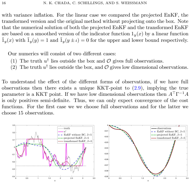
- [Assumptions versus numerical claims] All convergence theorems require A^T Γ^-1 A to be positive definite, a condition the authors themselves note in Remark 2.2 is typically false when n ≫ K. The numerical section includes low-dimensional observations for which A^T Γ^-1 A is only positive semidefinite, so the presented theorems do not cover those experiments; the phrase 'complete convergence analysis' therefore overstates the scope of the results.
minor comments (6)
- [§2.1, tensor product definition] The definition z1⊗z2(q) := ⟨z2,q⟩_{H2}·z2 appears to have a typo; the final factor should be z1, not z2.
- [§3.1, equation (3.2)] The Neumann expansion in equation (3.2) has all plus signs; the correct expansion of (h^{-1}Γ + C)^{-1} alternates in sign, starting with hΓ^{-1} - h^2 Γ^{-1} C Γ^{-1} + ... . The leading-order limit is unaffected, but the displayed series is incorrect.
- [§3.3.2, equation (3.12)] The last line of equation (3.12) repeats i = 1,...,m; it should read i = m+1,...,n.
- [§3.3.1, Remark 3.2] In the displayed computation of (C(u)+εI)_{ik}, the equality to 0 omits the εδ_{ik} contribution; only the off-diagonal part vanishes.
- [§3.3.3, Proposition 3.6 proof] The Grönwall-type estimate is misstated: from dV/dt ≤ -ε σ_min V one obtains V(t) ≤ V(0) exp(-σ_min ∫_0^t ε(s)ds), not the displayed integral inequality V(u0) ≥ ∫_0^t σ_min ε(s)ds V(ut).
- [General presentation] There are several typos, for example 'we we choose' in Section 4.1, and references [14] and [30] are listed as 'In preparation'; these should be updated or removed before any resubmission.
Circularity Check
No circularity: the convergence analysis extends independent continuous-time EKI and projected-gradient results without re-using its own conclusions as inputs.
full rationale
The paper's central derivation is the smoothed, variance-inflated projected EKI flow (3.13) and the claimed mean-square convergence to the KKT point u*_ι of the barrier problem (2.13). The continuous-time limit of the unconstrained EKI is imported from Schillings & Stuart [32], a published, externally reviewed, parameter-free result, and the projected-gradient/barrier framework is taken from Bertsekas [6,7] and Boyd-Vandenberghe [11]; none of these are unverified self-citations that smuggle in the paper's conclusion. The variance-inflation preconditioner D(u)=C(u)+εI is proposed from data-assimilation practice and Remark 3.2 verifies its structural property; it is not fitted to the target theorem. No parameter is tuned to a subset of data and then renamed a prediction, and no quantity is defined in terms of the convergence claim. The numerical section benchmarks against truth and against KKT points computed with fmincon, i.e. external comparators. The proof of Theorem 3.4 does contain a genuine algebraic gap: the displayed equality centers the empirical covariance at u*_ι rather than at the ensemble mean and drops the affine term involving ∇Φ(u*_ι), so the negativity of dV/dt is not established. That is a correctness flaw in the derivation, not a circular dependency: the claim is not equivalent to an input by construction, and the self-citations present in the paper are contextual or independently supported. Therefore no circularity is found.
Assumptions & free parameters
free parameters (4)
- ε (variance inflation constant) =
ε(t) = 1/(t^α + R), α = 0.75, R = 1 in numerics; ε > 0 in theory
- α =
0.75
- R =
1
- ι (log-barrier parameter) =
Not specified in numerics; taken large in theory
assumptions (4)
- domain assumption A^T Γ^-1 A is positive definite (strong observability).
- ad hoc to paper The discontinuous projected flow (3.4) can be replaced by the smoothed log-barrier flow (3.13), and convergence of the smoothed flow transfers to the algorithm.
- standard math The objective and the barrier function are strictly convex, yielding a unique global minimizer u*_ι of (2.13).
- domain assumption In the nonlinear setting, G(u) - G(ū) ≈ DG(ū)(u - ū).
Cite this review
Pith. "Pith review of On the Incorporation of Box-Constraints for Ensemble Kalman Inversion." pith.science (2026). https://pith.science/paper/WDG7ISHE
@misc{pith2026190800696,
  author       = {Pith},
  title        = {Pith review of: On the Incorporation of Box-Constraints for Ensemble Kalman Inversion},
  year         = {2026},
  howpublished = {\url{https://pith.science/paper/WDG7ISHE}},
  note         = {Machine review of arXiv:1908.00696}
}
read the original abstract
The Bayesian approach to inverse problems is widely used in practice to infer unknown parameters from noisy observations. In this framework, the ensemble Kalman inversion has been successfully applied for the quantification of uncertainties in various areas of applications. In recent years, a complete analysis of the method has been developed for linear inverse problems adopting an optimization viewpoint. However, many applications require the incorporation of additional constraints on the parameters, e.g. arising due to physical constraints. We propose a new variant of the ensemble Kalman inversion to include box constraints on the unknown parameters motivated by the theory of projected preconditioned gradient flows. Based on the continuous time limit of the constrained ensemble Kalman inversion, we discuss a complete convergence analysis for linear forward problems. We adopt techniques from filtering which are crucial in order to improve the performance and establish a correct descent, such as variance inflation. These benefits are highlighted through a number of numerical examples on various inverse problems based on partial differential equations.
Figures


Figures from the paper (7 more)


Reference graph
Works this paper leans on
-
[1]
N. Amor, G. Rasool, and N. C. Bouaynaya , Constrained state estimation - a review , ArXiv preprint, arxiv:807.03463, (2018)
work page 2018
-
[2]
J. L. Anderson , An adaptive covariance inflation error correction algorithm for ensemble filters, Tellus A, 59 (2007), pp. 210–224
work page 2007
-
[3]
, Spatially and temporally varying adaptive covariance inflation for ensemble filters , Tellus A, 61 (2009), pp. 72–83
work page 2009
-
[4]
K. Bergemann and S. Reich , A localization technique for ensemble Kalman filters , Quar- terly Journal of the Royal Meteorological Society, 136 (2010), pp. 701–707
work page 2010
- [5]
-
[6]
D. Bertsekas, Projected newton methods for optimization problems with simple constraints , SIAM Journal on Control and Optimization, 20 (1982), pp. 221–246
work page 1982
-
[7]
D. P. Bertsekas , Nonlinear programming, Athena Scientific, 2nd ed., Sept. 2008
work page 2008
-
[8]
On the stability of matrix-valued Riccati diffusions
A.N. Bishop and P. Del Moral, On the stability of matrix-valued Riccati diffusions, arXiv e-print, arXiv:1808.00235 (2018)
work page Pith review arXiv 2018
Show all 38 references
-
[9]
Bl ¨omker, C
D. Bl ¨omker, C. Schillings, and P. W acker , A strongly convergent numerical scheme from ensemble kalman inversion , SIAM Journal on Numerical Analysis, 56 (2018), pp. 2537 – 2562
2018
-
[10]
Bl ¨omker, C
D. Bl ¨omker, C. Schillings, P. W acker, and S. Weissmann , Well posedness and conver- gence analysis of the ensemble kalman inversion , Inverse Problems, 35 (2019), p. 085007
2019
-
[11]
Boyd and L
S. Boyd and L. V andenberghe , Convex Optimization , Cambridge University Press, New York, NY, USA, 2004
2004
-
[12]
N. K. Chada, M. A. Iglesias, L. Roininen, and A. M. Stuart , Parameterizations for ensemble Kalman inversion , Inverse Problems, 34 (2018), p. 055009
2018
-
[13]
X. Chen, J. D. Lee, X. T. Tong, and Y. Zhang , Statistical Inference for Model Parameters in Stochastic Gradient Descent , arXiv e-prints, (2016), p. arXiv:1610.08637
2016 arXiv
-
[14]
E. E. S. D. Albers, P-A. Blacquart and A. M. Stuart , Ensemble Kalman methods with constraints, In preparation, (2019)
2019
-
[15]
H. Engl, M. Hanke, and A. Neubauer , Regularization of Inverse Problems , Mathematics and Its Applications, Springer Netherlands, 2000
2000
-
[16]
Evensen , The ensemble Kalman filter: theoretical formulation and practical implemen- tation, Ocean Dynamics, 53 (2003), pp
G. Evensen , The ensemble Kalman filter: theoretical formulation and practical implemen- tation, Ocean Dynamics, 53 (2003), pp. 343–367. 22 N. K. CHADA, C. SCHILLINGS, AND S. WEISSMANN
2003
-
[17]
Evensen , Data Assimilation: The Ensemble Kalman Filter , Earth and Environmental Science, Springer Berlin Heidelberg, 2009
G. Evensen , Data Assimilation: The Ensemble Kalman Filter , Earth and Environmental Science, Springer Berlin Heidelberg, 2009
2009
-
[18]
M. A. Iglesias , A regularizing iterative ensemble Kalman method for PDE-constrained in- verse problems, Inverse Problems, 32 (2016), p. 025002
2016
-
[19]
M. A. Iglesias, K. Law, and A. M. Stuart , Ensemble Kalman methods for inverse prob- lems, Inverse Problems, 29 (2013), p. 045001
2013
-
[20]
Kaipio and E
J. Kaipio and E. Somersalo , Statistical and Computational Inverse Problems , Applied Mathematical Sciences, Springer New York, 2006
2006
-
[21]
Kandepu, L
R. Kandepu, L. Imsland, and B. A. Foss , Constrained state estimation using the unscented Kalman filter, 16th Mediterranean Conference on Control and Automation, (2008)
2008
-
[22]
Kelly, K
D. Kelly, K. Law, and A. M. Stuart , Well-posedness and accuracy of the ensemble Kalman filter in discrete and continuous time , Nonlinearity, 27 (2014), p. 2579
2014
-
[23]
Kelly, A
D. Kelly, A. J. Majda, and X. T. Tong , Concrete ensemble Kalman filters with rigorous catastrophic filter divergence, Proceedings of the National Academy of Sciences, (2015)
2015
-
[24]
Kwiatkowski and J
E. Kwiatkowski and J. Mandel , Convergence of the square root ensemble Kalman filter in the large ensemble limit , SIAM/ASA Journal on Uncertainty Quantification, 3 (2015), pp. 1–17
2015
-
[25]
K. Law, A. M. Stuart, and K. Zygalakis , Data Assimilation: A Mathematical Introduc- tion, Texts in Applied Mathematics, Springer International Publishing, 2016
2016
-
[26]
Le Gland, V
F. Le Gland, V. Monbet, and V.-D. Tran , Large sample asymptotics for the ensemble Kalman filter, Research Report RR-7014, INRIA, 2009
2009
-
[27]
Li and A
G. Li and A. C. Reynolds , Iterative ensemble Kalman filters for data assimilation , Society of Petroleum Engineers, (2009)
2009
-
[28]
D. M. Livings, S. L. Dance, and N. K. Nichols , Unbiased ensemble square root filters , Physica D: Nonlinear Phenomena, 237 (2008), pp. 1021 – 1028
2008
-
[29]
B. K. P. Hungerlander and F. Rendl , Regularization of inverse problems via box con- strained minimization, ArXiv preprint arXiv:1807.11316, (2018)
2018 arXiv
-
[30]
Reich , Data assimilation, Acta Numerica, in preparation, (2019)
S. Reich , Data assimilation, Acta Numerica, in preparation, (2019)
2019
-
[31]
Reich and C
S. Reich and C. J. Cotter , Probabilistic Forecasting and Bayesian Data Assimilation, 2014
2014
-
[32]
Schillings and A
C. Schillings and A. M. Stuart , Analysis of the ensemble Kalman filter for inverse prob- lems, SIAM Journal on Numerical Analysis, 55 (2017), pp. 1264–1290
2017
-
[33]
Schmidt, D
M. Schmidt, D. Kim, and S. Sra , Projected newton-type methods in machine learning , (2013)
2013
-
[34]
Shikhman and O
V. Shikhman and O. Stein , Constrained optimization: Projected gradient flows , Journal of Optimization Theory and Applications, 140 (2009), pp. 117–130
2009
-
[35]
Simon , Kalman filtering with state constraints: a survey of linear and nonlinear algo- rithms, 4 (2009), pp
D. Simon , Kalman filtering with state constraints: a survey of linear and nonlinear algo- rithms, 4 (2009), pp. 1303–1318
2009
-
[36]
A. M. Stuart, Inverse problems: A bayesian perspective, Acta Numerica, 19 (2010), pp. 451– 559
2010
-
[37]
M. K. Tippett, J. L. Anderson, C. H. Bishop, T. M. Hamill, and J. S. Whitaker , Ensemble square root filters , Monthly Weather Review, 131 (2003), pp. 1485–1490
2003
-
[38]
W ang, Y
D. W ang, Y. Chen, and X. Cai , State and parameter estimation of hydrologic models using the constrained ensemble Kalman filter , Monthly Resources Research, 45 (2009). Department of Statistics and Applied Probability, National University of Singa- pore, 119077, Singapore E-ma...
2009
Reviewed August 14, 2026 · model on record in the stance chip above.
Discussion (0). Continue with ORCID to comment.