REVIEW 2 major objections 3 minor 1 cited by
Universal Reconfiguration of Facet-Connected Modular Robots by Pivots: The $O(1)$ Musketeers
T0 review · 2 major / 3 minor · reviewed 2026-08-14 · deepseek-v4-flash
Pith's one-line read The paper proves that five extra helper modules suffice to reconfigure any facet-connected square-grid robot into any other shape of the same size using pivot moves, with an O(n^2)-move algorithm that is worst-case optimal.
desk verdict Genuinely new and important result; the five-musketeer bound has a real unproved step (d≤6 in Lemma 13) that a referee should pin down before acceptance. read the letter →
The pith
A machine-rendered reading of the paper's core claim, the machinery that carries it, and where it could break.
The reading
What carries the argument
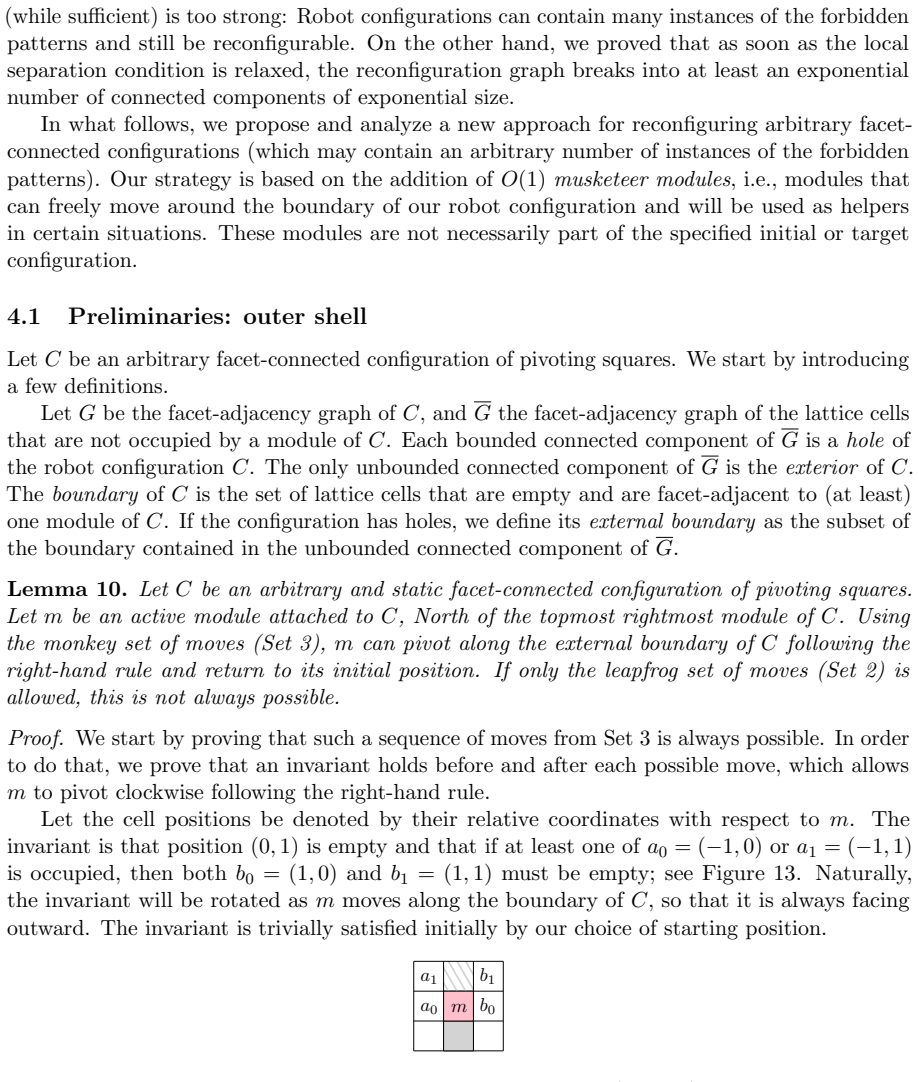
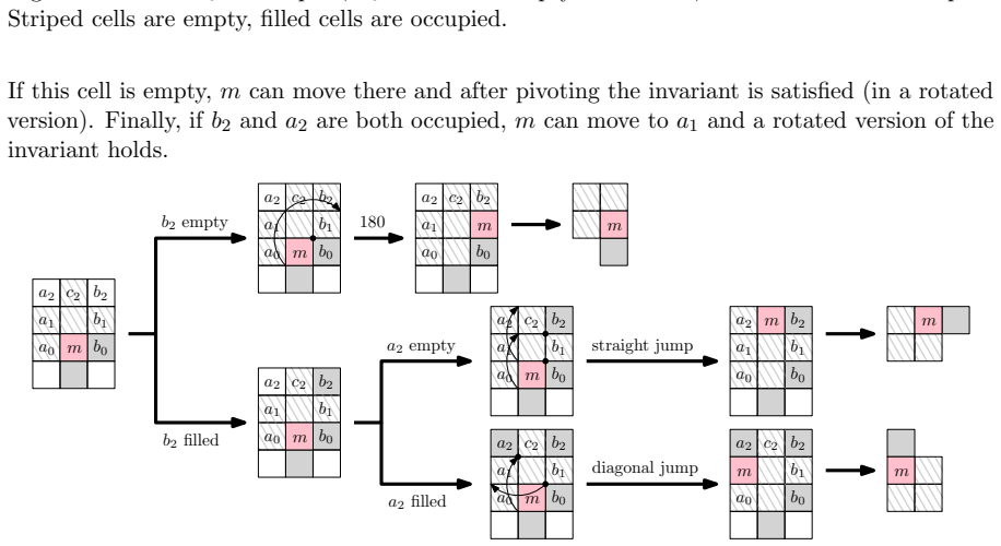
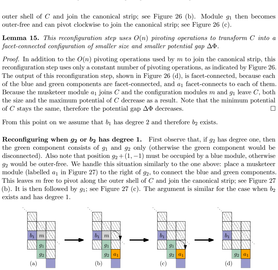
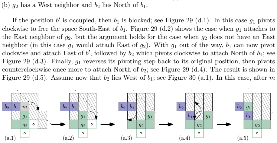
The device that carries the argument is the outer-shell traversal: a module placed just outside the robot's boundary can pivot clockwise around the entire outer shell using only straight monkey jumps, following the right-hand rule, and return to its start (Lemma 10). Progress is measured by the lexicographic potential $\Phi(m)=(x+y,x)$: the algorithm repeatedly removes the maximum-potential module into a canonical strip. When that module is a cut vertex joining two components, the bridging procedure slides a small window $S$ along the boundary until it touches both components, then places up to five helper modules to reconnect them; the case analysis is organized by the distance $d$ between the closest green and blue modules adjacent to the bridge rectangle.
What would settle it
Simulate Algorithm 1 on small facet-connected configurations, say up to 20 squares, and for each maximum-potential module compute the grid distance between the closest pair of modules from the two components cut by that module; finding any configuration with distance 7 or greater, or any bridge needing a sixth helper, would refute the claim that five musketeers always suffice.
Extended reading notes
Core claim
The central claim is Theorem 20: Algorithm 1 turns any facet-connected configuration of n pivot modules in the square grid into a straight strip of n modules, and by reversing the move sequence any strip into any target shape, using O($n^{2}$) monkey pivot moves and at most five added helper modules; the O($n^{2}$) count is worst-case optimal. The route through the strip means the result is equivalent to proving that the reconfiguration graph of n modules plus up to five free helpers is connected. On the way, the paper proves that with no helpers the graph is far from connected, with an exponential number of components, some of exponential size and some isolated rigid configurations. It also defines three nested families of pivot moves, restrictive, leapfrog, and monkey, and shows the resulting reconfiguration graphs are strictly different.
Load-bearing premise
The load-bearing premise is the assertion in the bridging lemma that the grid distance between the closest pair of modules from the two separated pieces can only be 2 through 6; if the distance could be 7 or more, the five-helper case analysis would not cover it and five helpers might not suffice.
Editorial extensions
If this is right
- Any two facet-connected configurations of the same number of modules become mutually reachable once five spare modules are allowed, because both can be reduced to the same canonical strip and the moves reversed.
- The move count O(n^2) is asymptotically optimal: some pairs of configurations, such as a vertical strip and a horizontal strip, force each module to travel distance $\Theta(n)$, giving an $\Omega(n^2)$ lower bound.
- The unassisted reconfiguration graph's exponential fragmentation shows why previous forbidden-pattern restrictions were not just an artifact of proof technique; without helpers, universal reconfiguration is impossible.
- The algorithm only needs straight monkey jumps, not diagonal ones, so the guarantee covers pivot hardware that can perform the simpler straight jump.
- The three move models are genuinely different: some configurations are reachable under monkey moves but not leapfrog, and some under leapfrog but not restrictive.
Reading between the lines
- I infer that if a counterexample to the assertion that the bridging distance $d$ is at most 6 exists, the framework would not collapse: it would merely push the helper constant upward, and the same outer-shell strategy would likely give universality with a larger fixed number of helpers.
- I infer that the outer-shell and bridging ideas are portable to cube lattices in three dimensions, where the bridge window would need more helpers; the paper itself lists this as an open direction, and I would expect the constant to grow with dimension.
- I infer that because the algorithm is explicit, a simulator could test the five-helper promise directly on small random configurations; the bridged cases $d=2$ through $d=6$ are all drawn, so one can check whether the figures cover every local pattern that actually occurs.
- I infer that the musketeer idea suggests a general principle for lattice reconfiguration: a constant number of freely placeable agents can bypass deadlocks even when the unassisted state space is exponentially disconnected, which may apply to other lattices and move sets.
Signed reviews
Editorial analysis
A structured set of objections, weighed in public.
Referee Report
Summary. The paper studies reconfiguration of facet-connected square-grid modular robots under pivot moves. It introduces three nested move sets (restrictive, leapfrog, and monkey) and proves that they give strictly different reconfiguration graphs. It shows that configurations with a certain forbidden pattern can have exponentially many connected components, including exponentially many singleton (rigid) components in some models. The main algorithmic result, Theorem 20, claims that any two facet-connected configurations of n modules can be reconfigured into each other using at most five additional 'musketeer' modules and O(n^2) monkey-move pivoting steps, which is worst-case optimal. The algorithm repeatedly moves outer-free modules along the external boundary to a canonical strip; when no outer-free module exists, a bridging procedure uses up to five musketeer modules to break the cut vertex and make progress. The proof of the constant five rests on a case analysis over a distance parameter d defined in the bridging procedure (Lemma 13).
Significance. If correct, the main theorem is a substantial advance: it removes the forbidden-pattern admissibility restriction from prior pivot-reconfiguration results and gives a precise constant number of helper modules, together with a matching worst-case move bound. The model separations and the exponential connected-component results are also valuable contributions. The paper is self-contained, the algorithm is concrete, and the potential-function framework is a clear structure for proving termination and monotonicity. However, the proof of the constant five rests on an unproved bound on the parameter d in Lemma 13, so the central claim is not yet fully established.
major comments (2)
- [Section 4.3.2, Lemma 13] The proof of Lemma 13 states without argument that 'It is easy to see that d can only be 2, 3, 4, 5, or 6.' This is a load-bearing claim because the subsequent case analysis in Figures 19–23 covers only these values, and the maximum number of musketeer modules needed in the bridging procedure is determined by the largest d considered. The rectangle R is the union of two 3x3 squares, so modules facet-adjacent to R on opposite sides can in principle be at L1 distance larger than 6. The precondition that the configuration has no outer-free modules may rule this out, but no proof is supplied. If d could be 7 or larger, the bridging procedure would require more than five musketeer modules in at least one case, contradicting Theorem 20. The authors must either prove d <= 6 or modify the argument.
- [Section 4.3.2, bridging case analysis (Figures 19–23)] The case analyses for d = 2 through 6 are presented almost entirely through figures, and the text asserts for each case that the indicated 'must' occupancies follow from the absence of outer-free modules and that the displayed musketeer sequences are feasible. The completeness of the enumeration—up to rotations and reflections, and the listed options—is not argued formally. Because the correctness and the helper bound of Lemma 13 depend on this enumeration being exhaustive, the proof needs either a formal symmetry argument or a more explicit derivation of each case. Without this, the reader cannot verify that all configurations with the stated invariants are covered.
minor comments (3)
- [Figure 13 caption] The caption says 'If a1 or a2 are occupied, then both b1 and b2 are empty', but the proof text defines the relevant positions as a0, a1, b0, and b1. The caption labels should be updated to match the proof.
- [Theorem 20 statement] The phrase 'into a canonical strip of the same size, adding at most five extra modules' is ambiguous: the final strip contains n original modules plus up to five helpers, so the total length is n + h with h <= 5. This should be stated precisely.
- [Section 4.3.2, Observation 12] The observation that the outer shell has exactly two green-blue changes of color, one at m, is used to justify the traversal of the square S, but its proof is not given. A short justification would improve readability.
Circularity Check
No circularity: the central derivation is self-contained; the unproved d<=6 bound in Lemma 13 is a proof gap, not a circular reduction.
full rationale
Walking the derivation chain: the paper defines three pivot-move models and proves separations between them using explicit configurations and connectivity arguments; the reconfiguration graph results in Section 3 are proved directly from the definitions and external prior work. Section 4 introduces the outer shell via Lemma 10, whose right-hand-rule traversal proof is carried out case-by-case in the text. The bridging procedure in Section 4.3.2 enumerates cases d=2 through d=6 with explicit musketeer placements and proves connectivity and potential arguments for each. Lemmas 14-19 handle the remaining neighborhood configurations, and Theorem 20 combines these into the O(n^2) bound with the earth-moving lower bound. No fitted parameter is later called a prediction; no input definition is equivalent to the output theorem; and no load-bearing claim is justified solely by a self-citation. The references to prior pivot-move work [20], the idea of helper modules [12], and the cactus graph [7] are all external to the present author set, so self-citation is not an issue. The only notable weakness is the sentence in Lemma 13, 'It is easy to see that d can only be 2, 3, 4, 5, or 6,' which asserts the key upper bound on the green-blue distance without proof. That is a genuine missing argument and a correctness risk for the five-musketeer sufficiency claim, but it is not circularity: the bound is not assumed as an input, derived from a fit, or obtained by renaming a prior result. A proof gap is different from a self-referential reduction, so the circularity score remains 0.
Assumptions & free parameters
assumptions (3)
- domain assumption Module motion is restricted to pivot moves on a square lattice with facet-connectivity maintenance.
- domain assumption Up to five extra modules (musketeers) may be added to the configuration and are not part of the start or goal shapes.
- standard math The active module's right-hand-rule traversal of the boundary is well-defined on the square lattice outer shell.
Cite this review
Pith. "Pith review of Universal Reconfiguration of Facet-Connected Modular Robots by Pivots: The $O(1)$ Musketeers." pith.science (2026). https://pith.science/paper/WGJFU23H
@misc{pith2026190807880,
  author       = {Pith},
  title        = {Pith review of: Universal Reconfiguration of Facet-Connected Modular Robots by Pivots: The $O(1)$ Musketeers},
  year         = {2026},
  howpublished = {\url{https://pith.science/paper/WGJFU23H}},
  note         = {Machine review of arXiv:1908.07880}
}
abstract
We present the first universal reconfiguration algorithm for transforming a modular robot between any two facet-connected square-grid configurations using pivot moves. More precisely, we show that five extra "helper" modules ("musketeers") suffice to reconfigure the remaining $n$ modules between any two given configurations. Our algorithm uses $O(n^2)$ pivot moves, which is worst-case optimal. Previous reconfiguration algorithms either require less restrictive "sliding" moves, do not preserve facet-connectivity, or for the setting we consider, could only handle a small subset of configurations defined by a local forbidden pattern. Configurations with the forbidden pattern do have disconnected reconfiguration graphs (discrete configuration spaces), and indeed we show that they can have an exponential number of connected components. But forbidding the local pattern throughout the configuration is far from necessary, as we show that just a constant number of added modules (placed to be freely reconfigurable) suffice for universal reconfigurability. We also classify three different models of natural pivot moves that preserve facet-connectivity, and show separations between these models.
Figures



Figures from the paper (29 more)









Forward citations
Cited by 1 Pith paper
-
Stress-Sharing for Decentralized Fault Repair in Modular Spacecraft
A local-information, connectivity-safe pivot policy restores most connectivity in simulated modular spacecraft after random damage, although full reconnection collapses with size and fault density.
Reference graph
Works this paper leans on
-
[20]
C. Sung, J. Bern, J. Romanishin, and D. Rus. Reconfiguration planning for pivoting cube modular robots. In Proceedings of the IEEE International Conference on Robotics and Automation (ICRA), pages 1933–1940, 2015
work page 1933
-
[1]
Z. Abel and S. D. Kominers. Pushing hypercubes around. CoRR, abs/0802.3414, 2008. arXiv:0802.3414
work page Pith review arXiv 2008
-
[2]
B. K. An. EM-Cube: cube-shaped, self-reconfigurable robots sliding on structure surfaces. In Proc. IEEE International Conference on Robotics and Automation (ICRA), pages 3149–3155, 2008
work page 2008
-
[3]
N. Ayanian, P. J. White, ´A. H´ al´ asz, M. Yim, and V. Kumar. Stochastic control for self- assembly of XBots. In Proceedings of the ASME International Design Engineering Technical Conferences and Computers and Information in Engineering Conference , 2008
work page 2008
-
[4]
N. M. Benbernou. Geometric algorithms for reconfigurable structures . PhD thesis, Mas- sachusetts Institute of Technology, 2011
work page 2011
-
[5]
S. Chennareddy, A. Agrawal, and A. Karuppiah. Modular self-reconfigurable robotic systems: a survey on hardware architectures. Journal of Robotics, 2017(5013532), 2017
work page 2017
-
[6]
G. S. Chirikjian. Kinematics of a metamorphic robotic system. In Proc. IEEE International Conference on Robotics and Automation (ICRA) , volume 1, pages 449–455, 1994
work page 1994
-
[7]
A. Dumitrescu and J. Pach. Pushing squares around. Graphs and Combinatorics , 22(1):37– 50, 2006
work page 2006
Show all 23 references
-
[8]
Fitch, Z
R. Fitch, Z. Butler, and D. Rus. Reconfiguration planning for heterogeneous self- reconfiguring robots. In Proc. IEEE/RSJ International Conference on Intelligent Robots and Systems (IROS) , volume 3, pages 2460–2467, 2003
2003
-
[9]
Hemmerling
A. Hemmerling. Labyrinth problems – labyrinth-searching abilities of automata , volume 14 of Teubner-Texte zur Mathematik (TTZM) . Springer-Verlag, 1989
1989
-
[10]
Kurokawa, S
H. Kurokawa, S. Murata, E. Yoshida, K. Tomita, and S. Kokaji. A 3-D self-reconfigurable structure and experiments. In Proc. IEEE/RSJ International Conference on Intelligent Robots and Systems (IROS) , volume 2, pages 860–865, 1998
1998
-
[11]
Larkworthy and S
T. Larkworthy and S. Ramamoorthy. A characterization of the reconfiguration space of self-reconfiguring robotic systems. Robotica, 29(1):73–85, 2011
2011
-
[12]
Michail, G
O. Michail, G. Skretas, and P. G. Spirakis. On the transformation capability of feasible mechanisms for programmable matter. J. Comput. Syst. Sci. , 102:18–39, 2019
2019
-
[13]
Murata, H
S. Murata, H. Kurokawa, and S. Kokaji. Self-assembling machine. In Proc. IEEE In- ternational Conference on Robotics and Automation (ICRA) , volume 1, pages 441–448, 1994
1994
-
[14]
Murata, E
S. Murata, E. Yoshida, A. Kamimura, H. Kurokawa, K. Tomita, and S. Kokaji. M-TRAN: self-reconfigurable modular robotic system. IEEE/ASME Transactions on Mechatronics, 7(4):431–441, 2002. 28
2002
-
[15]
Nguyen, L
A. Nguyen, L. J. Guibas, and M. Yim. Controlled module density helps reconfiguration planning. In Algorithmic and Computational Robotics: New Dimensions (WAFR) , pages 23–25. A. K. Peters, 2001
2001
-
[16]
E. H. Østergaard, K. Kassow, R. Beck, and H. H. Lund. Design of the ATRON lattice-based self-reconfigurable robot. Autonomous Robots, 21(2):165–183, 2006
2006
-
[17]
Rus and M
D. Rus and M. Vona. A physical implementation of the self-reconfiguring crystalline robot. In Proc. IEEE International Conference on Robotics and Automation (ICRA) , volume 2, pages 1726–1733, 2000
2000
-
[18]
Salemi, M
B. Salemi, M. Moll, and W.-M. Shen. SUPERBOT: a deployable, multi-functional, and modular self-reconfigurable robotic system. In Proc. IEEE/RSJ International Conference on Intelligent Robots and Systems (IROS) , pages 3636–3641, 2006
2006
-
[19]
K. Stoy, D. Brandt, and D. J. Christensen. Self-reconfigurable robots: an introduction. MIT Press, 2010
2010
-
[21]
Unsal, H
C. Unsal, H. Kiliccote, and P. Khosla. I(CES)-Cubes: a modular self-reconfigurable bipartite robotic system. In Proc. SPIE Conference on Mobile Robots and Autonomous Systems , volume 3839, pages 258–269. SPIE, 1999
1999
-
[22]
M. Yim, W. Shen, B. Salemi, D. Rus, M. Moll, H. Lipson, E. Klavins, and G. S. Chirikjian. Modular self-reconfigurable robot systems. IEEE Robotics & Automation Magazine, 14(1):43– 52, 2007
2007
-
[23]
Zykov, A
V. Zykov, A. Chan, and H. Lipson. Molecubes: an open-source modular robotic kit. In IROS-2007 Self-Reconfigurable Robotics Workshop, 2007. 29
2007
Reviewed August 14, 2026 · model on record in the stance chip above.
Discussion (0). Continue with ORCID to comment.