REVIEW 3 major objections 5 minor 83 references
Bondi accretion disk luminosity around neutral and charged Simpson-Visser spacetimes
T0 review · 3 major / 5 minor · reviewed 2026-08-06 · deepseek-v4-flash
Pith's one-line read This paper claims that the Simpson-Visser regularization length ℓ and electric charge Q shift the Bondi sonic radius, accretion rate, and luminosity of inflowing gas, offering a double observational marker to distinguish regular black…
desk verdict The exponential-density branch is a sound extension of Bondi accretion to Simpson-Visser spacetimes, but the barotropic branch, which drives the headline marker claim, has no valid sonic point and its reported radii are artifacts. read the letter →
The pith
A machine-rendered reading of the paper's core claim, the machinery that carries it, and where it could break.
The reading
What carries the argument
The machinery is the relativistic Bondi–Michel critical point system. From the conservation of energy flux and mass flux, the velocity equation is written in terms of the variable $V^2=d\ln(P+\rho)/d\ln\rho-1$, and the critical (sonic) point is fixed by the simultaneous vanishing of the two brackets, giving $V_c^2=1/(2\sqrt{x^2+\ell^2}/M-3)$ and $u_c^2=M/(2\sqrt{x^2+\ell^2})$ for the neutral case, with charged generalizations involving $Q$. Equating these critical quantities with the fluid-specific velocity law—$u^2=C_4^2/(1+w)^2-A(x)$ for the barotropic fluid, $u=C_3/(\rho(x^2+\ell^2))$ for the exponential profile—locates the sonic radius $x_c$, which is then converted into the mass accretion rate $\dot M=-4\pi(x^2+\ell^2)(P+\rho)u\sqrt{u^2+A}$ and the luminosity $L=\eta_{\rm eff}\dot M$. This chain from metric to velocity profile to observable is what carries the claim that ℓ and $Q$ leave measurable fingerprints in accretion flows.
What would settle it
Compute $V^2=d\ln(P+\rho)/d\ln\rho-1$ for $P=w\rho$: since the specific enthalpy $(P+\rho)/\rho=1+w$ is constant, $V^2\equiv 0$, and the first critical condition $V_c^2=u_c^2/(u_c^2+A)$ then forces $u_c=0$, so no finite sonic point exists. Solving the authors' equations (14a)–(14b) directly with $V^2=0$ for the constants in Tables I and IV and checking whether any positive $x_c$ remains would settle whether the barotropic sonic radii and the claimed barotropic shifts are physical; the exponential-density results are unaffected by this check.
Extended reading notes
Core claim
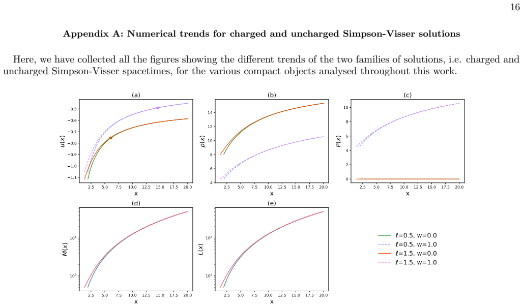
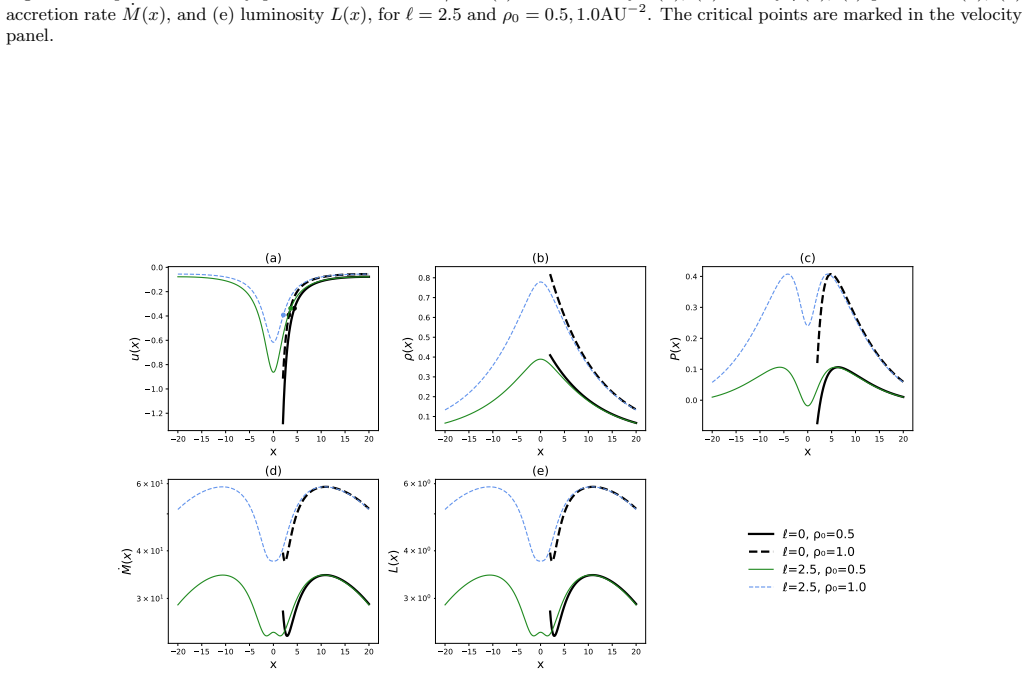
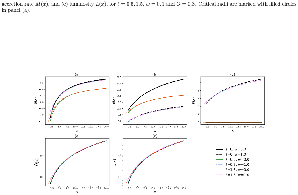
On the paper's own terms, the discovery is that the Bondi accretion observables encode the regularization parameter ℓ and the electric charge $Q$. Solving the Michel-type critical point system for the neutral Simpson-Visser metric $A(x)=1-2M/\sqrt{x^2+\ell^2}$, the authors find sonic radii that decrease slightly with ℓ for the barotropic fluid (deviations below roughly 1.5% from Schwarzschild) but shift substantially for the exponential density profile, reaching about 18% at $\rho_0=0.5\,\mathrm{AU}^{-2}$ and 36% at $\rho_0=1.0\,\mathrm{AU}^{-2}$ in the wormhole regime $\ell=2.5$. In the charged spacetime $A(x)=1-2M/\sqrt{x^2+\ell^2}+Q^2/(x^2+\ell^2)$ with $Q=0.3$, the sonic radius shifts by fractions of a percent for the black-hole cases and by up to about 8% (barotropic, $w=0$) or 35% (exponential, $\rho_0=1$) in the wormhole case relative to Reissner-Nordström. The critical inflow velocity $u_c$ is unchanged to numerical precision in every configuration, and near-horizon velocities are similar across solutions, whereas ℓ acts mainly on the critical point's position and $Q$ slightly dampens the near-horizon inflow velocity in the barotropic case. The paper concludes that ℓ and $Q$ together provide a double observational marker to distinguish these spacetimes from standard black holes.
Load-bearing premise
The load-bearing premise is that the standard Michel-type critical point system, which locates the sonic point by equating critical and fluid velocities, remains valid for a constant-$w$ barotropic fluid with $P=w\rho$; if that system does not admit a finite nonzero sonic radius for the chosen constants, then the barotropic critical radii reported in the tables would be artifacts rather than physical predictions.
Editorial extensions
If this is right
- A measured sonic radius that deviates from the Schwarzschild value by more than a few percent cannot be produced by the barotropic fluid models considered, but is naturally produced by an exponential-density flow in the wormhole regime, so the fluid model matters for interpreting any observed shift.
- If the accretion flow around a candidate compact object is consistent with an exponential density profile, deviations in $x_c$ of order 18–36% in the wormhole regime would indicate Simpson-Visser-type regularization rather than a Schwarzschild or Reissner-Nordström geometry.
- Because $Q$ shifts the sonic radius by only fractions of a percent in black-hole cases, a measurement of $x_c$ alone cannot fix $Q$; the combination of $x_c$ and the near-horizon inflow velocity (damped by $Q$ in the barotropic case) is needed to separate the two parameters.
- The insensitivity of the critical inflow velocity $u_c$ to both ℓ and $Q$ means velocity measurements at the sonic point are not a diagnostic; the diagnostic power lies in the location of the sonic point and in the luminosity and accretion-rate profiles.
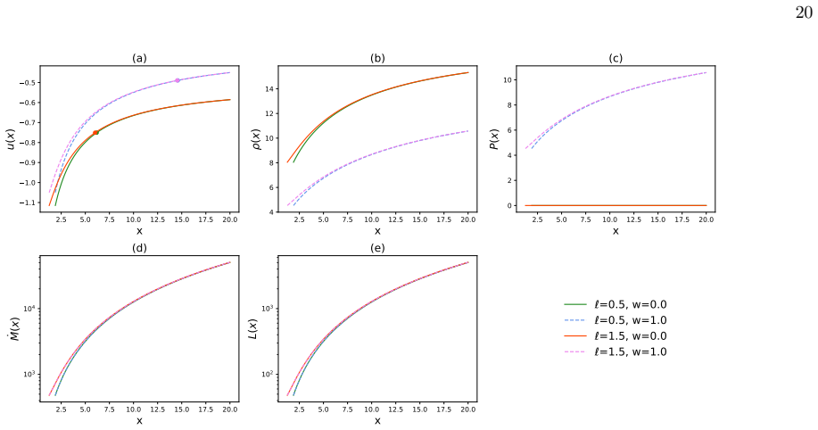
- For barotropic fluids, the near-overlap of all solutions (deviations below about 1.5%) implies that if the accreting matter is stiff or dust-like, standard and regular black holes are hard to separate with Bondi observables alone.
Reading between the lines
- One extension the paper does not pursue is testing how sensitive these shifts are to the specific choice of regular geometry; repeating the same Bondi calculation for Bardeen or Hayward metrics would show whether the ℓ-induced sonic shifts are a generic feature of regular black holes or specific to the Simpson-Visser coordinate choice.
- The exponential-density results are the more robust channel for the proposed marker, because the constant-$w$ barotropic critical point construction can degenerate (for $P=w\rho$ the sound-speed combination vanishes identically); an independent derivation of the sonic condition for such fluids would clarify whether the barotropic trend is physical or an artifact of the chosen integration constants
- A practical test of the double marker would be to fit the predicted luminosity and sonic-radius patterns to low-luminosity galactic nuclei, using the exponential profile as a proxy for dark-matter-contaminated environments; real accretion disks add angular momentum, magnetic fields, and radiative transfer that the spherically symmetric Bondi model omits, so the observed luminosity would need de-pr
- If the near-horizon velocity insensitivity holds, spectral or interferometric measurements of inflow speed would be blind to ℓ and $Q$, pushing observational searches toward the sonic point location and bolometric luminosity instead.
Editorial analysis
A structured set of objections, weighed in public.
Referee Report
Summary. The manuscript studies relativistic Bondi accretion in neutral and charged Simpson-Visser spacetimes, treating two fluid models: a constant-w barotropic fluid (P = wρ) and a fluid with an exponential density profile. The authors derive conservation equations, locate critical (sonic) points, integrate velocity/density/pressure profiles, and compute accretion rates and luminosities for Schwarzschild, regular black hole, and wormhole regimes. They conclude that the regularization parameter ℓ and the charge Q shift the sonic radius and modify accretion observables, proposing these shifts as a double observational marker for distinguishing regular black holes and wormholes from Schwarzschild and Reissner-Nordström solutions.
Significance. The core question—whether Bondi accretion observables can distinguish Simpson-Visser geometries from their classical counterparts—is timely and, if answered correctly, would be a useful contribution to the phenomenology of regular black holes. The manuscript presents a clear derivation of the conservation equations and an extensive set of numerical results, and the exponential-density branch appears internally consistent: a direct evaluation of V² at the tabulated exponential critical points satisfies the critical-point condition. However, the barotropic branch, which underpins the double-marker claim, is invalid because a constant-w equation of state makes the sound-speed variable V² vanish identically, so the critical-point system admits no finite positive-radius solution. The reported barotropic critical radii, accretion-rate deviations, and luminosity deviations are therefore artifacts rather than physical predictions, and the central observational claim is unsupported.
major comments (3)
- [§III.A, Eqs. (12)–(14); Tables I and IV] For the assumed equation of state P = wρ with constant w, the variable defined in Eq. (12) is identically zero: V² = d ln(P+ρ)/d ln ρ − 1 = d ln((1+w)ρ)/d ln ρ − 1 = 1 − 1 = 0. With V_c² = 0, Eq. (14a) forces u_c² = 0, and Eq. (14b) reduces to A′(x_c) = 0. For the neutral Simpson-Visser metric A′(x) = 2Mx/(x²+ℓ²)^{3/2}, which vanishes only at x = 0 (and is non-zero at x=0 for ℓ=0); for the charged metric with Q = 0.3 and the tabulated ℓ values, A′ also does not vanish at any positive radius used in the tables. Thus the critical radii reported in Tables I and IV do not solve the critical-point system derived by the authors. The barotropic columns of these tables and the corresponding figures are not supported by the equations in the paper.
- [Eq. (20); Table I] Equation (20) is algebraically inconsistent with the condition it claims to encode, namely the equality of Eq. (15b) and Eq. (18) at x = x_c. A direct derivation yields r_c = 3M(1+w)²/[2((1+w)² − C4²)], which is negative for the values used in Table I (C4 > 1+w), so no positive-radius solution exists for those constants. For ℓ=0, w=1, C4=2.09, the printed Eq. (20) gives x_c ≈ 4.04, whereas Table I reports 16.13; for w=0, C4=1.05, Eq. (20) gives x_c ≈ 3.82, again not 16.13. The tabulated values appear to come from the unsquared expression with an additional sign error. The barotropic critical radii, critical velocities, and all downstream accretion-rate and luminosity deviations are therefore not credible.
- [§V–§VI; Tables I–VI] The comparison of different geometries is not controlled with respect to the integration constants. The text states that the constants C_i are chosen to ensure the existence of a physical sonic point, and indeed C4 differs between the w=0 and w=1 cases (Tables I and IV) and C3 differs between the two exponential-density cases (Tables II and V). Since the critical radius depends sensitively on these constants, the percentage deviations in Tables III and VI cannot be attributed to ℓ and Q alone; they partly reflect the different boundary conditions chosen for each configuration. Even setting aside the barotropic inconsistency, the claim of a 'double observational marker' requires a common asymptotic boundary condition across the geometries being compared, which is not specified or implemented. This affects the quantitative predictions in both fluid models.
minor comments (5)
- [§V.A, paragraph after Fig. 2] The sentence 'from Eq. (21), it appears clear that the dependence on w is very weak' cites the wrong equation: Eq. (21) is the exponential-density velocity, not the barotropic expression; the dependence on w for the barotropic case should be discussed via Eq. (18).
- [Table II caption] The caption says 'C=10, C4 = 2.1', but the symbol C is not defined and the text uses C1 for the energy-flux constant; this should read C1=10.
- [Eq. (27) and §V] The luminosity formula in Eq. (27) uses η_eff, while the text and tables use η = 0.1; the notation should be unified.
- [§IV and §V] The units are inconsistent as written: M = 1 AU, Q = 0.3 (presumably in units of M but not stated), and ρ0 is given in AU^{-2}; please state the unit conventions explicitly for Q and ρ0.
- [Figures in Appendix A] The figure legends are missing the ℓ symbol (e.g., '=0.5, w=0.0' instead of 'ℓ=0.5, w=0.0'), which makes the plots difficult to read.
Circularity Check
Barotropic critical radii are artifacts: with P=wρ, V²≡0 makes the critical-point system unsolvable, and the reported x_c values are produced by hand-tuned constants C4, so the claimed ℓ/Q markers are not independent predictions.
-
fitted input called prediction
[Sec. III A 'Critical points', Eq. (20); Sec. V, Tables I]
"V 2 = d ln(P + ρ) d ln ρ − 1 ... P (x) = wρ(x) ... To find the critical point ... equate the expression of the velocity at the critical point, Eq. (15b), with its generic counterpart for the barotropic case, Eq. (18), evaluated at x = xc ... The result reads xc = ± s 3M 2(1 + w)2 2(C2 4 − (1 + w)2) ! − ℓ2 ... All integration constants, denoted by Ci, are chosen to ensure the existence of a physical sonic (critical) point."
For constant w, P+ρ=(1+w)ρ, so Eq. (12) gives V²=1−1=0 identically. The paper's own critical-point system (14a)-(14b) then forces u_c=0 and A′(x_c)=0, which has no finite solution for the Simpson-Visser or Reissner-Nordström metrics. The barotropic critical radius is instead obtained from the separate velocity equality defining Eq. (20), not from the critical-point system. Since C4 is freely chosen per (ℓ,w) 'to ensure the existence of a physical sonic point', the tabulated x_c values in Table I are not predictions of the spacetime model: they are restatements of the fitted C4 values.
-
fitted input called prediction
[Sec. IV A 'Barotropic fluid', Eq. (30); Sec. VI, Table IV]
"Barotropic fluid. Equating u2 c to the barotropic velocity expression, Eq. (18), leads to ... which has to be solved numerically for each ( ℓ, w) couple, since the presence of Q does not allow for analytical outcomes."
The charged barotropic branch inherits the same inconsistency: P=wρ with constant w makes V² in Eq. (12) vanish identically, so the charged critical-point condition (29a) cannot be satisfied at any finite radius. Equation (30) is again an imposed equality between the critical velocity expression and the barotropic velocity, not a solution of the critical-point system. With C4 already selected to force sonic points in the uncharged case, the additional 'modest shifts' attributed to Q in Table IV are generated by solving an equation that the model itself says has no critical point. Hence the claimed double observational marker (ℓ plus Q) is not an independent derivation but a consequence of the imposed velocity equality and hand-picked constants.
full rationale
The paper's general Bondi conservation equations and the exponential-density-profile branch are self-contained: the exponential critical radii are obtained by solving the stated algebraic conditions for each fixed C3, and no self-citation chain is load-bearing. However, the central barotropic claims fail internal consistency: for P=wρ, Eq. (12) gives V²=0 identically, which makes the critical-point system (14a)-(14b) unsolvable at finite radius. The paper bypasses this by imposing a separate velocity equality (Eqs. 20 and 30) and by tuning C4 per (ℓ,w) to 'ensure the existence of a physical sonic point'. The reported barotropic critical radii, velocities, accretion rates, luminosities, and the ℓ/Q shifts derived from them therefore reduce to the chosen integration constants rather than to predictions of the spacetime geometry. This is partial circularity concentrated in the barotropic sector, hence score 6 rather than 0-2; the exponential sector and the formal framework are not similarly compromised.
Assumptions & free parameters
free parameters (9)
- Simpson-Visser length ℓ =
0.5, 1.5, 2.5 (plus 0 for Schwarzschild/RN)
- Barotropic EoS parameter w =
0 and 1
- Exponential density profile amplitude ρ0 =
0.5 and 1.0 AU⁻²
- Exponential density profile radius r0 =
10 AU
- Integration constant C4 (barotropic) =
2.09, 1.05, 2.10, 1.12 (varies by case)
- Integration constant C3 (mass flux) =
1.9, 2.1, 3.0 (varies by case)
- Charge Q =
0.3
- Efficiency parameter η =
0.1
- Mass M =
1 AU
assumptions (4)
- domain assumption Stationary, radial, spherically symmetric perfect fluid accretion
- domain assumption Mass flux conservation J^µ = ρ u^µ is assumed
- ad hoc to paper The Michel critical point system with V² as defined applies to each fluid
- domain assumption The exponential density profile is a complete fluid model
Cite this review
Pith. "Pith review of Bondi accretion disk luminosity around neutral and charged Simpson-Visser spacetimes." pith.science (2026). https://pith.science/paper/WHBVTDJL
@misc{pith2026250721580,
  author       = {Pith},
  title        = {Pith review of: Bondi accretion disk luminosity around neutral and charged Simpson-Visser spacetimes},
  year         = {2026},
  howpublished = {\url{https://pith.science/paper/WHBVTDJL}},
  note         = {Machine review of arXiv:2507.21580}
}
abstract
We investigate relativistic Bondi accretion in the Simpson-Visser spacetime, which, via a single parameter $\ell$, interpolates between the Schwarzschild, regular black hole, extremal and wormhole regimes. First, we analyze the neutral Simpson-Visser geometry, recovering Schwarzschild at $\ell=0$, and then its charged extension of the Reissner-Nordstr\"om metric. In both these cases, we derive the conservation equations and analyze two representative fluid models: a barotropic perfect fluid and a constituent with an exponential density profile. By varying the parameters across regimes, we locate critical (sonic) points and integrate velocity, density and pressure profiles. While near-horizon inflow velocities are similar across the different solutions, we find that the critical radius and the resulting accretion rates and luminosities severely change, depending on the value of the parameter and type of fluid. Remarkably, the barotropic and exponential cases exhibit different trends in the outer regions. Moreover, by extending the analysis to the charged SV spacetime, we find that the presence of a central charge $Q$ produces additional, albeit modest, shifts in the sonic radius which, in combination with those induced by the regularization parameter $\ell$, could provide a double observational marker. In particular, while $\ell$ acts predominantly on the position of the critical point, in the barotropic fluid case, the electromagnetic contribution of $Q$ slightly dampens the inflow velocity near the horizon.
Figures


Figures from the paper (13 more)




Reference graph
Works this paper leans on
-
[1]
Exponential density profile 9
-
[2]
Bondi accretion for charged Simpson-Visser spacetime 10 A
Quantifying deviations from the Schwarzschild solution 10 VI. Bondi accretion for charged Simpson-Visser spacetime 10 A. Regular black hole accretion 11 Barotropic equation of state 11 Exponential density profile 12 B. Wormholes accretion 12
-
[3]
Barotropic equation of state 12
-
[4]
Exponential density profile 13 arXiv:2507.21580v1 [gr-qc] 29 Jul 2025 2
work page Pith review arXiv 2025
-
[5]
Final outlooks 14 Acknowledgments 15 A
Deviations from the Reissner-Nordstr¨ om solution 14 VII. Final outlooks 14 Acknowledgments 15 A. Numerical trends for charged and uncharged Simpson-Visser solutions 16 References 24 I. INTRODUCTION Black holes (BHs) are among the most intriguing ob- jects predicted by general relativity and solutions to Einstein’s equations. While many observations in re...
-
[6]
The classical solution, depicted by black lines, closely resembles the RBH cases with small ℓ. Inflow velocity, density, and pressure profiles, shown in panels (a), (b), and (c), respectively, begin to diverge near the center. The critical radius increases by up to∼ 6 for moderate values of ℓ. Unlike the barotropic model, the exponential profile is less s...
-
[7]
In panel (a), the radial velocity of the Schwarzschild solution rises steeply near the horizon, whereas the worm- hole solutions feature a smoother gradient. Notably, the Schwarzschild profiles nearly coincide with the wormhole ones in the dust case, w = 0, albeit not for stiff matter. The critical radius xc in the wormhole configuration is slightly large...
-
[8]
Exponential density profile The wormhole case with an exponential density profile is shown in Fig. 7. The inflow velocity, panel (a), is again split into two sets of curves depending on the value of ρ0. The velocity decreases outward and remains symmetrical with respect to the throat. Near x = 0, the falloff is smoother than in BH cases, especially for hi...
Show all 83 references
-
[9]
Quantifying deviations from the Schwarzschild solution Above, our analyses focused on discrepancies among solutions and, in particular, using the Schwarzschild BH. It appears convenient to quantify how much the SV scenarios differ from the simplest spherically-symmetric soluti...
-
[10]
In panel (a), the velocity profiles show the same qual- itative behaviour as in the neutral wormhole case
Barotropic equation of state Figure 13 presents the charged wormhole accretion pro- files for barotropic fluids. In panel (a), the velocity profiles show the same qual- itative behaviour as in the neutral wormhole case. The inflow velocities decrease symmetrically on either si...
-
[11]
The velocity profiles in panel (a) remain largely unaf- fected by the presence of charge, with trends mirroring the neutral case
Exponential density profile Figure 15 shows the exponential accretion solutions for the charged wormhole configuration. The velocity profiles in panel (a) remain largely unaf- fected by the presence of charge, with trends mirroring the neutral case. Due to the absence of a hor...
-
[12]
The location of the event horizon shifts by up to 36% for ℓ = 1 .5
Deviations from the Reissner-Nordstr¨ om solution For the barotropic model, the critical radius xc shows deviations below 1% for RBHs and ∼ 1% for the worm- hole regimes with w = 0 and ∼ 8% for the other case. The location of the event horizon shifts by up to 36% for ℓ = 1 .5....
-
[13]
B. P. Abbott et al. (LIGO Scientific, Virgo), Phys. Rev. Lett. 116, 061102 (2016), 1602.03837
2016 arXiv
-
[14]
Akiyama et al
K. Akiyama et al. (Event Horizon Telescope), Astrophys. J. Lett. 875, L1 (2019), 1906.11238
2019 arXiv
-
[15]
S. W. Hawking and R. Penrose, Proc. Roy. Soc. Lond. A 314, 529 (1970)
1970
-
[16]
Hawking and R
S. Hawking and R. Penrose, The Nature of Space and Time (New in Paper) (Princeton University Press, 1996), ISBN 9780691145709, URL http://www.jstor.org/stable/j.ctt7szq2
1996
-
[17]
A. D. Sakharov, Soviet Journal of Experimental and Theoretical Physics 22, 241 (1966)
1966
-
[18]
E. B. Gliner, Soviet Journal of Experimental and Theoretical Physics 22, 378 (1966)
1966
-
[19]
Bardeen, in Proceedings of the 5th International Conference on Gravitation and the Theory of Relativity (1968), p
J. Bardeen, in Proceedings of the 5th International Conference on Gravitation and the Theory of Relativity (1968), p. 87
1968
-
[20]
C. Lan, H. Yang, Y. Guo, and Y.-G. Miao, Int. J. Theor. Phys. 62, 202 (2023), 2303.11696
2023 arXiv
-
[21]
Bueno, P
P. Bueno, P. A. Cano, and R. A. Hennigar, Phys. Lett. B 861, 139260 (2025), 2403.04827
2025 arXiv
-
[22]
Giamb` o and O
R. Giamb` o and O. Luongo, Class. Quant. Grav.41, 125005 (2024), 2308.10060
2024 arXiv
-
[23]
Corona, R
D. Corona, R. Giamb` o, and O. Luongo, Int. J. Geom. Meth. Mod. Phys. 21, 2440019 (2024), 2402.18997
2024 arXiv
-
[24]
S. A. Hayward, Phys. Rev. Lett. 96, 031103 (2006), gr-qc/0506126
2006 arXiv
- [26]
-
[27]
Ansoldi, in Conference on Black Holes and Naked Singularities (2008), 0802.0330
S. Ansoldi, in Conference on Black Holes and Naked Singularities (2008), 0802.0330
2008 arXiv
-
[28]
K. A. Bronnikov, Phys. Rev. D 63, 044005 (2001), gr-qc/0006014
2001 arXiv
- [29]
-
[30]
Kurmanov, K
Y. Kurmanov, K. Boshkayev, T. Konysbayev, O. Luongo, N. Saiyp, A. Urazalina, G. Ikhsan, and G. Suliyeva, Phys. Dark Univ. 46, 101566 (2024), 2404.15437
2024 arXiv
-
[31]
G. J. Olmo, J. L. Rosa, D. Rubiera-Garcia, and D. Saez-Chillon Gomez, Class. Quant. Grav.40, 174002 (2023), 2302.12064
2023 arXiv
-
[32]
J. a. L. Rosa and D. Rubiera-Garcia, Phys. Rev. D 106, 084004 (2022), 2204.12949
2022 arXiv
- [33]
- [34]
- [35]
-
[36]
Carballo-Rubio et al., JCAP 05, 003 (2025), 2501.05505
R. Carballo-Rubio et al., JCAP 05, 003 (2025), 2501.05505
2025 arXiv
-
[37]
Bambi, ed., Regular Black Holes
C. Bambi, ed., Regular Black Holes. Towards a New Paradigm of Gravitational Collapse , Springer Series in Astrophysics and Cosmology (Springer, 2023), ISBN 978-981-99-1595-8, 978-981-99-1598-9, 978-981-99-1596-5, 2307.13249
2023 arXiv
- [38]
-
[39]
Bambhaniya, S
P. Bambhaniya, S. K, K. Jusufi, and P. S. Joshi, Phys. Rev. D 105, 023021 (2022), 2109.15054
2022 arXiv
-
[40]
Murodov, K
S. Murodov, K. Badalov, J. Rayimbaev, B. Ahmedov, and Z. Stuchl ´ ık, Symmetry16, 109 (2024)
2024
-
[41]
Alencar, A
G. Alencar, A. Duran-Cabac´ es, D. Rubiera-Garcia, and D. S´ aez-Chill´ on G´ omez, Phys. Rev. D 111, 104020 (2025), 2501.03909
2025 arXiv
- [42]
-
[43]
S. I. Kruglov, Annalen Phys. 528, 588 (2016), 1607.07726
2016 arXiv
-
[44]
S. I. Kruglov, Annals Phys. 378, 59 (2017), 1703.02029
2017 arXiv
-
[45]
Gullu and S
I. Gullu and S. H. Mazharimousavi, Phys. Scripta 96, 045217 (2021), 2009.08665
2021 arXiv
-
[46]
Guerrero, G
M. Guerrero, G. J. Olmo, D. Rubiera-Garcia, and D. S´ aez-Chill´ on G´ omez, Phys. Rev. D106, 044070 (2022), 2205.12147
2022 arXiv
-
[47]
Combi, H
L. Combi, H. Yang, E. Gutierrez, S. C. Noble, G. E. Romero, and M. Campanelli, Phys. Rev. D 109, 103034 (2024), 2405.06900
2024 arXiv
-
[48]
M. V. d. S. Silva and M. E. Rodrigues, Int. J. Theor. Phys. 63, 101 (2024), 2404.15792
2024 arXiv
- [49]
-
[50]
F. S. N. Lobo, A. Simpson, and M. Visser, Phys. Rev. D 101, 124035 (2020), 2003.09419
2020 arXiv
-
[51]
Duran-Cabac´ es, D
A. Duran-Cabac´ es, D. Rubiera-Garcia, and D. S´ aez-Chill´ on G´ omez (2025), 2506.10814
2025 arXiv
-
[52]
J. Lu, S. Yang, Y. Zhang, L. Yang, and M. Xu, Nucl. Phys. B 1010, 116775 (2025), 2403.19942
2025 arXiv
-
[53]
S. Yang, J. Lu, X. Yu, and J. Xu, Class. Quant. Grav. 42, 045006 (2025), 2403.17454
2025 arXiv
-
[54]
Luongo (2025), 2504.09987
O. Luongo (2025), 2504.09987
2025
-
[55]
Bondi, Mon
H. Bondi, Mon. Not. Roy. Astron. Soc. 112, 195 (1952)
1952
-
[56]
F. C. Michel, Astrophys. Space Sci. 15, 153 (1972)
1972
-
[57]
Sofue, Mass Distribution and Rotation Curve in the Galaxy (Springer Netherlands, Dordrecht, 2013), pp
Y. Sofue, Mass Distribution and Rotation Curve in the Galaxy (Springer Netherlands, Dordrecht, 2013), pp. 985–1037, ISBN 978-94-007-5612-0, URL https://doi.org/10.1007/978-94-007-5612-0_19
2013 doi
- [58]
-
[59]
Boshkayev, A
K. Boshkayev, A. Idrissov, O. Luongo, and D. Malafarina, Mon. Not. Roy. Astron. Soc. 496, 1115 (2020), 2006.01269
2020 arXiv
-
[60]
Sofue, M
Y. Sofue, M. Honma, and T. Omodaka, Publ. Astron. Soc. Jap. 61, 227 (2009), 0811.0859
2009 arXiv
- [61]
- [62]
- [63]
-
[64]
J. A. d. Freitas Pacheco (2011), 1109.6798
2011 arXiv
-
[65]
C. B. Richards, T. W. Baumgarte, and S. L. Shapiro, Mon. Not. Roy. Astron. Soc. 502, 3003 (2021), [Erratum: Mon.Not.Roy.Astron.Soc. 506, 3935 (2021)], 2101.08797
2021 arXiv
- [66]
-
[67]
Babichev, V
E. Babichev, V. Dokuchaev, and Y. Eroshenko, Phys. Rev. Lett. 93, 021102 (2004), gr-qc/0402089
2004 arXiv
-
[68]
A. C. Alfano and O. Luongo (2025), 2501.15233
2025 arXiv
-
[69]
A. C. Alfano, O. Luongo, and M. Muccino, JHEAp 46, 100348 (2025), 2411.04878
2025 arXiv
-
[70]
A. C. Alfano, O. Luongo, and M. Muccino, JCAP 12, 055 (2024), 2408.02536
2024 arXiv
-
[71]
Carloni, O
Y. Carloni, O. Luongo, and M. Muccino, Phys. Rev. D 111, 023512 (2025), 2404.12068
2025 arXiv
- [72]
-
[73]
Anaya-Galeana, O
J. Anaya-Galeana, O. Luongo, and H. Quevedo, Phys. Dark Univ. 46, 101672 (2024), 2407.02429
2024 arXiv
-
[74]
Carloni, O
Y. Carloni, O. Luongo, and M. Muccino (2025), 2506.11531
2025
-
[75]
P. K. S. Dunsby, O. Luongo, M. Muccino, and V. Pillay, Phys. Dark Univ. 46, 101563 (2024), 2403.17880
2024 arXiv
-
[76]
P. K. S. Dunsby, O. Luongo, and M. Muccino, Phys. Rev. D 109, 023510 (2024), 2308.15776
2024 arXiv
-
[77]
Luongo and H
O. Luongo and H. Quevedo, Int. J. Mod. Phys. D 23, 1450012 (2014)
2014
-
[78]
P. K. S. Dunsby, O. Luongo, and L. Reverberi, Phys. Rev. D 94, 083525 (2016), 1604.06908
2016 arXiv
-
[79]
Kurmanov, K
E. Kurmanov, K. Boshkayev, R. Giamb` o, T. Konysbayev, O. Luongo, D. Malafarina, and H. Quevedo, Astrophys. J.925, 210 (2022), 2110.15402
2022 arXiv
-
[80]
Boshkayev, T
K. Boshkayev, T. Konysbayev, Y. Kurmanov, O. Luongo, and D. Malafarina, Astrophys. J. 936, 96 (2022), 2205.04208
2022 arXiv
-
[81]
Boshkayev, T
K. Boshkayev, T. Konysbayev, E. Kurmanov, O. Luongo, D. Malafarina, and H. Quevedo, Phys. Rev. D 104, 084009 (2021), 2106.04932
2021 arXiv
- [82]
-
[83]
Frank, A
J. Frank, A. King, and D. J. Raine, Accretion Power in Astrophysics: Third Edition (Cambridge University Press, 2002)
2002
- [84]
Reviewed August 6, 2026 · model on record in the stance chip above.
Discussion (0). Sign in to comment.