REVIEW 2 major objections 5 minor 70 references
An Assessment of Organics Detection and Characterization on the Surface of Europa with Infrared Spectroscopy
T0 review · 2 major / 5 minor · reviewed 2026-08-07 · deepseek-v4-flash
Pith's one-line read Europa Clipper's MISE spectrometer can detect trace organic molecules on Europa at abundances below one percent, using Bayesian model comparison, and can constrain abundances of spectrally rich species even amid overlapping features from…
desk verdict A valuable, well-scoped simulation study of MISE's ability to detect trace organics, but the sub-percent BMC thresholds are same-model self-consistency numbers, not yet tested against forward-model mismatch. read the letter →
The pith
A machine-rendered reading of the paper's core claim, the machinery that carries it, and where it could break.
The reading
What carries the argument
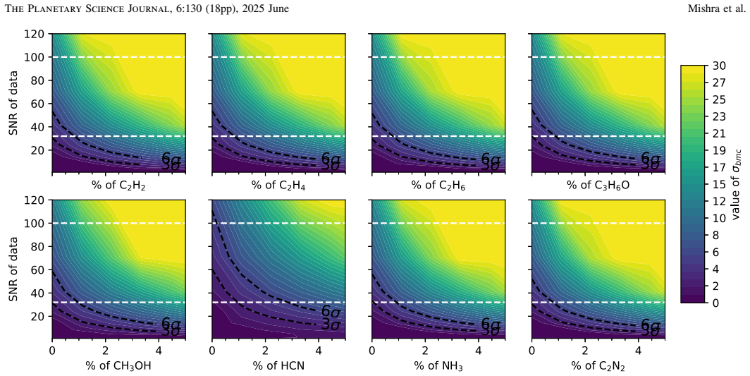
The load-bearing machinery is the Hapke bidirectional reflectance model, an analytical formula for the radiance factor of a particulate regolith in terms of incidence, emergence, and phase angles, porosity, and the single-scattering albedo of the intimate mixture; single-scattering albedos are computed from laboratory optical constants of each species via the equivalent-slab approximation, so that abundances translate into spectral features. On top of this forward model sit two detection metrics: the feature-strength statistic σ_fs, the average amplitude of a species' chosen absorption features divided by the local noise, and the Bayesian model comparison statistic σ_bmc, obtained by computing the Bayesian evidence for a model with the candidate species versus a model without it (via the dynesty nested-sampling algorithm) and converting the Bayes factor to a σ significance. The paper's visualization tool, the "detectability heatmap," plots σ_fs or σ_bmc contoured over abundance on the x-axis and SNR on the y-axis, with instrument SNR limits and 3σ/6σ contours overlaid, which turns the detection question into a map that any instrument's capabilities can be checked against.
What would settle it
A laboratory blind test would settle the matter: prepare (or simulate, with a deliberately different generative model) a reflectance spectrum of an icy regolith containing a known organic at 1% abundance, degrade it to MISE's 10 nm resolution at SNR 50, and run the BMC retrieval with an end-member set that is imperfect in a known way (for example, amorphous instead of crystalline water ice, or a different grain-size distribution). If the detection significance drops below 3σ, or the recovered abundance is biased by more than 2σ, then the shared-model assumption is doing real work in the paper's thresholds.
Extended reading notes
Core claim
This paper establishes a quantitative detectability result for organics on Europa: given the spectral resolution (10 nm) and signal-to-noise (SNR ~30–100) that Europa Clipper's MISE spectrometer will deliver in the 3–5 μm window, trace organic molecules can be pulled out of a water-ice-dominated spectrum at far lower abundances than their weak band depths would suggest. Using simulated reflectance spectra built with the Hapke bidirectional reflectance model and laboratory optical constants at Europan temperatures, the authors show that HCN, C2N2, C2H4, and CH3OH reach the 3σ threshold near 5% abundance by feature strength alone, and that Bayesian model comparison—which exploits each species' effect on the whole continuum, not just its sharp lines—lowers the 3σ threshold below 1% abundance for all eight organics considered. In the 11-species mixture test, BMC detects every organic species in the presence of overlapping features and co-mingled oxides, and retrieves abundances within 2σ for the most spectrally rich species. The paper states plainly that these are idealized best-case numbers, since the simulated data and the retrieval model share the same photometric model and the same optical constants.
Load-bearing premise
The simulations assume the model that generates the data is the same model used to analyze it, down to the same photometric law and the same laboratory optical constants for every component; if a real Europa spectrum departs from those lab end-members in grain shape, temperature, phase, or hydration state, the sub-percent detection thresholds could prove optimistic.
Editorial extensions
If this is right
- If these thresholds hold, MISE becomes the first instrument able to map organic composition across Europa's surface, letting scientists correlate specific molecules with lineae, chaos terrains, and other geologically young features where ocean-derived material may be exposed.
- The Bayesian approach converts a noise problem into signal: species with no single prominent feature can still be detected through their subtle imprint on the continuum, giving roughly a fivefold improvement in detection threshold over feature-strength analysis.
- In complex mixtures with overlapping features, BMC resolves species that would be ambiguous by eye—such as the shared ~4.26 μm absorption of HCN, C2N2, C2H2, C2H6, C3H6O, and CO2—and provides abundance constraints, not just detections, for spectrally rich species.
- The dilution-based instrument comparison implies that high spatial resolution, not raw SNR, is the decisive capability for finding localized organic patches: MISE's scaled SNR of 30–100 far exceeds the values below 1.1 estimated for Galileo/NIMS, Keck/NIRSPEC, and JWST/NIRSpec for a 100 km² deposit.
- Observation strategy matters: moderate incidence and emergence angles near 45°, larger grain sizes, and the choice of low-irradiation target regions all strengthen organic features, giving mission planning a physical basis for where and how to look.
Reading between the lines
- These thresholds are sensitivity ceilings, not performance guarantees: the simulations share the photometric model and optical constants between data and retrieval, so real-surface complications such as temperature-dependent end-members, hydration states, or non-50 μm grain distributions could push detection limits upward; reading them as upper bounds on capability is the safe interpretation until
- The detectability-heatmap tool is effectively a reusable instrument-design instrument: inverted, it can specify the SNR and resolution a future mission needs to claim a given detection threshold, and the same pipeline transfers to ESA's JUICE/MAJIS observations of Europa.
- A positive detection of organics at local abundances well above tenth-of-a-percent levels, following the reasoning the paper cites for CH2 groups, would argue for an endogenic source from Europa's ocean rather than meteoritic infall, making MISE's spatial resolution the key to an astrobiological claim.
- A natural stress test would be to run the same BMC pipeline on laboratory reflectance spectra of irradiated ice–organic mixtures, where the generative model is unknown by construction; if the retrieved abundances stay unbiased and detections stay above 3σ, the sub-percent claims are much harder to break.
Editorial analysis
A structured set of objections, weighed in public.
Referee Report
Summary. The paper presents a simulation-based feasibility study of detecting trace organic molecules on Europa's surface with near-infrared reflectance spectroscopy at MISE-like resolution and SNR. Using the Hapke bidirectional reflectance model with water ice plus one or more organic species (and, in one case, CO2 and SO2), the authors generate noisy spectra, then evaluate detectability by (i) the average strength of selected absorption features relative to noise (σ_fs) and (ii) Bayesian model comparison between a full model and a model with the candidate removed (σ_bmc). They produce abundance–SNR detectability heatmaps for eight organics, apply BMC to an 11-species mixture, examine sensitivity to geometry, grain size, and porosity, and compare MISE with other instruments using a dilution-based SNR scaling. The main conclusions are that sharp-featured species are detectable at ~5% abundance and SNR~100 via feature strength, and that BMC lowers the 3σ threshold to <1% abundance; in the 11-species mixture all organics are detected at moderate-to-strong significance, with abundances constrained for the spectrally richest species.
Significance. If the reported thresholds are taken as upper limits under idealized assumptions, the paper is a useful and timely contribution: it develops a clear, reusable framework (detectability heatmaps, BMC pipeline) for planning Europa Clipper/MISE observations, uses publicly available cryogenic optical constants, and is explicit about the idealized character of the simulations. The detectability-heatmap tool and the analysis of spectral confusion in a multi-species mixture are likely to be of practical use to the community. The main limitation is that the retrieval is validated on data generated with the same forward model and end-member optical constants, so the quantitative thresholds are self-consistency results until tested against model mismatch; this does not invalidate the framework but must be stated in the abstract.
major comments (2)
- [§3.2, §3.3, Abstract] The <1% BMC detection thresholds are established in a fully self-consistent setting: the simulated data are generated with the same Hapke photometric model and the same laboratory optical constants that are used in the retrieval (Section 2.1; the idealized nature is acknowledged in Sections 3.2 and 3.3). The paper's own sensitivity study (Section 3.4) varies geometry, grain size, and porosity for the forward spectra but does not inject any of these mismatches into the BMC calculation, so it does not quantify how much model–data mismatch is required to erase the sub-percent detection. Because the abstract states that BMC "pushes the 3σ detection threshold ... to <1% abundance" without the best-case caveat, this is a load-bearing gap for the mission-relevant claim. I request a quantitative robustness test—for example, generating data with a different porosity coefficient, a grain-size distribution, or perturbed end-member optical constants and recomputing σ_bmc for representative abundances and SNRs—and that the abstract and Conclusions state the conditions under which the thresholds hold.
- [§3.5, Eq. (8)] The dilution-based SNR scaling is presented as a quantitative comparison tool, but Equation (8) multiplies the area and bandwidth ratios linearly without derivation. For a photon-noise-limited observation, the signal from a sub-pixel feature is diluted by the area fraction f = A_feature/A_I, while the noise is determined by the total photon count from the whole pixel; the feature SNR therefore does not in general scale linearly with f. The absolute scaled SNRs in Table 2 and the "MISE uniquely capable" conclusion in Section 3.5 rest on this unvalidated scaling. I suggest deriving the scaling from a noise model or explicitly labeling Table 2 as an illustrative order-of-magnitude exercise rather than a quantitative prediction.
minor comments (5)
- [Abstract] Consider adding the phrase "under idealized photometric and end-member assumptions" to the sentences reporting the 5% and <1% detection thresholds, so that the abstract does not overstate the mission-level capability.
- [§3.3, Conclusion item 3] The statement that retrievals "go beyond detection to actually constraining abundances (to within 2σ of the true value)" is too broad; the same paragraph notes that HCN, CO2, and SO2 posteriors are only upper limits. Rephrase to say that abundances are constrained to within 2σ for the spectrally rich species.
- [§3.5, Table 2] The notation in Equation (8) and Table 2 is confusing: Δλ_I is used for the instrument channel width while the feature bandwidth is also described as 10 nm. Clarify the definitions and ensure the table columns match the equation symbols.
- [§3.4, Figure 12] The caption for Figure 12 says "porosity" but the plotted parameter appears to be the porosity coefficient K; state the range of K values used so that the reader can interpret the amplitude changes.
- [§2.3] The sentence explaining the Sellke/Trotta conversion is garbled in the text; please rewrite it to state explicitly that Equation (6) gives an upper bound on the p-value and Equation (7) then gives a lower bound on the detection significance, valid for p ≤ e^{-1}.
Circularity Check
No significant circularity: the shared forward model is a stated idealization and standard power-analysis setup, not a definitional equivalence.
full rationale
The paper's central claim is a detectability threshold computed from simulated spectra in which trace species are injected at known abundances and SNR. The retrieval and BMC use the same Hapke radiative-transfer model and the same laboratory optical constants as the data generator. This is a standard power-analysis or self-consistency setup, not a circular reduction: the detection threshold is a nonlinear function of the injected signal, the noise model, and the prior ranges, and it is not equivalent to any fitted parameter or to the input abundance by construction. The paper explicitly acknowledges the idealized nature of the exercise: Section 3.2 states "it is important to note that this is an idealized case, where the model components and the simulated data share the same photometric model and optical constants," and Section 3.3 repeats that "these results assume idealized conditions—accurate spectral end-members and perfect photometric modeling." Section 3.4 then defers inclusion of photometric nuisance parameters in the full BMC analysis to future work. These passages are limitations on external validity for real Europa data, not evidence that the derivation equals its inputs. The self-citations to Mishra et al. (2021a, 2021b) are methodological references to the Hapke implementation and Bayesian evidence framework; they are not load-bearing in the sense of importing an unverified uniqueness claim or smuggling in an ansatz. No fitted input is renamed as a prediction, and no known result is merely relabeled. The paper is appropriately scoped as a simulation feasibility study, and no circular step can be exhibited.
Assumptions & free parameters
free parameters (4)
- Regolith grain size =
50 μm
- Observation geometry angles =
i = e = 45°, g = 90°
- Dilution scaling feature area and bandwidth =
100 km2, 10 nm
- Porosity coefficient K =
1
assumptions (6)
- domain assumption The Hapke bidirectional reflectance model with a two-parameter Henyey-Greenstein phase function and porosity coefficient accurately represents Europa's regolith reflectance.
- domain assumption The equivalent slab approximation correctly computes single-scattering albedo for intimate mixtures from optical constants and grain size.
- domain assumption Laboratory optical constants measured at about 60-130 K for the trace species and water ice are valid for Europa's surface conditions.
- domain assumption Hydrated non-ice materials on Europa are spectrally similar to water ice beyond 3 μm and do not significantly affect the detectability conclusions.
- standard math Gaussian, independent measurement errors with SNR = reflectance / noise.
- domain assumption Uniform priors on abundance fractions (0-1) and grain sizes (10-1000 μm) in the Bayesian retrievals.
Cite this review
Pith. "Pith review of An Assessment of Organics Detection and Characterization on the Surface of Europa with Infrared Spectroscopy." pith.science (2026). https://pith.science/paper/WJUWVLNU
@misc{pith2026250601842,
  author       = {Pith},
  title        = {Pith review of: An Assessment of Organics Detection and Characterization on the Surface of Europa with Infrared Spectroscopy},
  year         = {2026},
  howpublished = {\url{https://pith.science/paper/WJUWVLNU}},
  note         = {Machine review of arXiv:2506.01842}
}
abstract
Organics, if they do exist on Europa, may only be present in trace amounts on the surface. NASA's upcoming mission Europa Clipper is going to provide global, high quality data of the surface of Europa in the near-infrared (NIR), specifically the 3-5~$\mu$m region, where organics are rich in spectroscopic features. In this work we investigate Europa Clipper's ability to constrain the abundance of selected trace species of interest that span different chemical bonds found in organics, such as C-H, C=C, C$\equiv$C, C=O and C$\equiv$N, via NIR spectroscopy in the 3-5~$\mu$m wavelength region. We simulate reflectance spectra of these trace species mixed with water ice, at varying SNR and abundance fractions. The evidence for the trace species in a mixture is evaluated using two approaches: 1) calculating average strength of absorption feature(s), and 2) Bayesian model comparison (BMC) analysis. Our simulations show that sharp and strong spectroscopic features of trace ($\sim 5\%$ abundance by number) organic species should be detectable at $> 3\sigma$ significance in Europa Clipper quality data. A BMC analysis pushes the $3\sigma$ detection threshold of trace species even lower to $<1 \%$ abundance. We also consider an example with all trace species mixed together, with overlapping features, and BMC is able to retrieve strong evidence for all of them and also provide constraints on their abundance. These results are promising for Europa Clipper's capability to detect trace organic species, which would allow correlations to be drawn between the composition and geological regions with possibly endogenic material.
Figures


Figures from the paper (10 more)




Reference graph
Works this paper leans on
-
[1]
Becker, T. M., Trumbo, S. K., Molyneux, P. M., et al. 2022, PSJ , 3, 129
work page 2022
-
[2]
Belgacem, I., Schmidt, F., & Jonniaux, G. 2020,Icar, 338, 113525
work page 2020
-
[3]
Belgacem, I., Schmidt, F., & Jonniaux, G. 2021,Icar, 369, 114631
work page 2021
- [4]
- [5]
-
[6]
Blaney, D. L., Hibbitts, C., Green, R. O., et al. 2023, LPSC,2806, 2472
work page 2023
-
[7]
Carlson, R. W., Calvin, W. M., Dalton, J. B., et al. 2009, Europa(Tucson, AZ: Univ. Arizona Press),283
work page 2009
-
[8]
Carnall, A. C. 2017, arXiv:1705.05165
arXiv 2017
Show all 70 references
-
[9]
A., Paranicas, C
Cassidy, T. A., Paranicas, C. P., Shirley, J. H., et al. 2013,P&SS , 77, 64
2013
-
[10]
1960, Radiative Transfer(New York: Dover),
Chandrasekhar, S. 1960, Radiative Transfer(New York: Dover),
1960
-
[11]
F., & Phillips, C
Chyba, C. F., & Phillips, C. B. 2001,PNAS , 98, 801
2001
-
[12]
N., Cruikshank, D
Clark, R. N., Cruikshank, D. P., Jaumann, R., et al. 2012,Icar, 218, 831
2012
-
[13]
N., Fanale, F
Clark, R. N., Fanale, F. P., & Zent, A. P. 1983,Icar, 56, 233
1983
-
[14]
Dalton, J. B. 2007,GeoRL, 34, L21205
2007
-
[15]
Dalton, J. B. 2010,SSRv , 153, 219
2010
-
[16]
B., Mogul, R., Kagawa, H
Dalton, J. B., Mogul, R., Kagawa, H. K., Chan, S. L., & Jamieson, C. S. 2003, AsBio, 3, 505
2003
-
[17]
B., Shirley, J
Dalton, J. B., Shirley, J. H., & Kamp, L. W. 2012,JGRE , 117, E03003 De Angelis, S., Tosi, F., Carli, C., et al. 2020,Icar, 357, 114165 De Angelis, S., Tosi, F., Carli, C., et al. 2021,Icar, 373, 114756
2012
-
[18]
2013,JGRE , 118, 534
Fernando, J., Schmidt, F., Ceamanos, X., et al. 2013,JGRE , 118, 534
2013
-
[19]
2016,JOSS , 1, 24
Foreman-Mackey, D. 2016,JOSS , 1, 24
2016
-
[20]
K., Coustenis, A., et al
Grasset, O., Dougherty, M. K., Coustenis, A., et al. 2013,P&SS , 78, 1
2013
-
[21]
P., & Carlson, R
Hand, K. P., & Carlson, R. W. 2012, JGRE , 117, E03008
2012
-
[22]
P., Carlson, R
Hand, K. P., Carlson, R. W., & Chyba, C. F. 2007, AsBio, 7, 1006
2007
-
[23]
P., Chyba, C
Hand, K. P., Chyba, C. F., Carlson, R. W., & Cooper, J. F. 2006,AsBio, 6, 463
2006
-
[24]
P., Chyba, C
Hand, K. P., Chyba, C. F., Priscu, J. C., et al. 2009, in Europa, ed. R. T. Pappalardo, W. B. McKinnon, & K. K. Khurana (Tucson, AZ: Univ. Arizona Press), 589
2009
-
[25]
P., & German, C
Hand, K. P., & German, C. R. 2018, NatGe, 11, 2
2018
-
[26]
P., Phillips, C
Hand, K. P., Phillips, C. B., Murray, A., et al. 2022,PSJ , 3, 22
2022
-
[27]
B., & McCord, T
Hansen, G. B., & McCord, T. B. 2008,GeoRL, 35, L01202
2008
-
[28]
1981, JGRB, 86, 3039
Hapke, B. 1981, JGRB, 86, 3039
1981
-
[29]
2021,Icar, 354, 114105
Hapke, B. 2021,Icar, 354, 114105
2021
-
[30]
R., Millman, K
Harris, C. R., Millman, K. J., van der Walt, S. J., et al. 2020,Natur, 585, 357
2020
-
[31]
R., Cassidy, T
Hendrix, A. R., Cassidy, T. A., Johnson, R. E., Paranicas, C., & Carlson, R. W. 2011, Icar, 212, 736
2011
-
[32]
G., & Greenstein, J
Henyey, L. G., & Greenstein, J. L. 1941,ApJ, 93, 70
1941
-
[33]
M., & Pappalardo, R
Howell, S. M., & Pappalardo, R. T. 2020, NatCo, 11, 1311
2020
-
[34]
Hunter, J. D. 2007,CSE , 9, 90
2007
-
[35]
1998, The Theory of Probability(Oxford: Oxford Univ
Jeffreys, H. 1998, The Theory of Probability(Oxford: Oxford Univ. Press)
1998
-
[36]
A., & Prockter, L
Kattenhorn, S. A., & Prockter, L. M. 2014,NatGe, 7, 762
2014
-
[37]
2019,MNRAS , 489, 5231
Khawaja, N., Postberg, F., Hillier, J., et al. 2019,MNRAS , 489, 5231
2019
-
[38]
2016, Jupyter Notebooks – A Publishing Format for Reproducible Computational Work/f_lows, in Positioning and Power in Academic Publishing: Players, Agents and Agendas, ed
Kluyver, T., Ragan-Kelley, B., Pérez, F., et al. 2016, Jupyter Notebooks – A Publishing Format for Reproducible Computational Work/f_lows, in Positioning and Power in Academic Publishing: Players, Agents and Agendas, ed. F. Loizides & B. Schmidt(Amsterdam: IOS Press), 87
2016
-
[39]
Lapotre, M. G. A., Ehlmann, B. L., & Minson, S. E. 2017,JGRE , 122, 983
2017
-
[40]
2016,AJ, 151, 163
Ligier, N., Poulet, F., Carter, J., Brunetto, R., & Gourgeot, F. 2016,AJ, 151, 163
2016
-
[41]
Lunine, J. I. 2017,AcAau, 131, 123
2017
-
[42]
M., Sandford, S
Mastrapa, R. M., Sandford, S. A., Roush, T. L., Cruikshank, D. P., & Dalle Ore, C. M. 2009,ApJ, 701, 1347
2009
-
[43]
B., Carlson, R
McCord, T. B., Carlson, R. W., Smythe, W. D., et al. 1997, Sci, 278, 271
1997
-
[44]
B., Hansen, G
McCord, T. B., Hansen, G. B., Clark, R. N., et al. 1998,JGR, 103, 8603
1998
-
[45]
J., & Charnley, S
Mumma, M. J., & Charnley, S. B. 2011, ARA&A, 49, 471
2011
-
[46]
2018, JGRE , 123, 2564
Poch, O., Cerubini, R., Pommerol, A., Jost, B., & Thomas, N. 2018, JGRE , 123, 2564
2018
-
[47]
2023, LPSC,2806, 1310 17 The Planetary Science Journal, 6:130(18pp ), 2025 June Mishra et al
Poulet, F., Piccioni, G., Langevin, Y., et al. 2023, LPSC,2806, 1310 17 The Planetary Science Journal, 6:130(18pp ), 2025 June Mishra et al
2023
-
[48]
M., Shirley, J
Prockter, L. M., Shirley, J. H., Dalton, J. B., & Kamp, L. 2017,Icar, 285, 27
2017
-
[49]
C., & Hedman, M
Quick, L. C., & Hedman, M. M. 2020, Icar, 343, 113667
2020
-
[50]
1999,Icar, 139, 159
Quirico, E., Douté, S., Schmitt, B., et al. 1999,Icar, 139, 159
1999
-
[51]
1997,Icar, 127, 354
Quirico, E., & Schmitt, B. 1997,Icar, 127, 354
1997
-
[52]
Schenk, P. M. 2020, ApJ, 892, L12
2020
-
[53]
2015,Icar, 260, 73
Schmidt, F., & Fernando, J. 2015,Icar, 260, 73
2015
-
[54]
2018, Solid Spectroscopy Hosting Architecture of Databases and Expertise(SSHADE ), doi:10.26302/ SSHADE /MIRABELLE
Schmitt, B., Bollard, P., Albert, D., et al. 2018, Solid Spectroscopy Hosting Architecture of Databases and Expertise(SSHADE ), doi:10.26302/ SSHADE /MIRABELLE
2018
-
[55]
1994,Icar, 111, 79
Schmitt, B., de Bergh, C., Lellouch, E., et al. 1994,Icar, 111, 79
1994
-
[56]
Solar System Ices
Schmitt, B., Quirico, E., Trotta, F., et al. 1998, in Solar System Ices: Based on Reviews Presented at the Int. Symp. “Solar System Ices” (Dordrecht: Kluwer),199
1998
-
[57]
J., & Berger, J
Sellke, T., Bayarri, M. J., & Berger, J. O. 2001,Am. Stat., 55, 62
2001
-
[58]
B., Hand, K
Sparks, W. B., Hand, K. P., McGrath, M. A., et al. 2016,ApJ, 829, 121
2016
-
[59]
Speagle, J. S. 2020,MNRAS , 493, 3132
2020
-
[60]
R., Tamppari, L
Spencer, J. R., Tamppari, L. K., Martin, T. Z., & Travis, L. D. 1999,Sci, 284, 1514
1999
-
[61]
2008,ConPh , 49, 71
Trotta, R. 2008,ConPh , 49, 71
2008
- [62]
-
[63]
E., & Davis, M
Trumbo, S., Brown, M. E., & Davis, M. R. 2023, Complete NIRSpec Coverage of Europa's Surface: CO2, Salt hydrates, and the Potential for Unexpected Discovery, JWST Proposal, Cycle 2, 4023, STScI
2023
-
[64]
K., & Brown, M
Trumbo, S. K., & Brown, M. E. 2023, Sci, 381, 1308
2023
-
[65]
K., Brown, M
Trumbo, S. K., Brown, M. E., Fischer, P. D., & Hand, K. P. 2017, AJ, 153, 250
2017
-
[66]
K., Brown, M
Trumbo, S. K., Brown, M. E., & Hand, K. P. 2019, AJ, 158, 127
2019
-
[67]
J., Helfenstein, P., & Buratti, B
Verbiscer, A. J., Helfenstein, P., & Buratti, B. J. 2013, in The Science of Solar System Ices, ed. M. S. Gudipati & J. Castillo-Rogez (New York: Springer),47
2013
-
[68]
B., Hand, K
Villanueva, G., Hammel, H. B., Hand, K. P., et al. 2017, Probing the Sub- surface Oceans of Europa and Enceladus with JWST, JWST Proposal, Cycle 1, 1250, STScI
2017
-
[69]
L., Hammel, H
Villanueva, G. L., Hammel, H. B., Milam, S. N., et al. 2023, Sci, 381, 1305
2023
-
[70]
E., et al
Virtanen, P., Gommers, R., Oliphant, T. E., et al. 2020,NatMe, 17, 261 18 The Planetary Science Journal, 6:130(18pp ), 2025 June Mishra et al
2020
Reviewed August 7, 2026 · model on record in the stance chip above.
Discussion (0). Continue with ORCID to comment.