REVIEW 4 major objections 5 minor 64 references
Learning with springs and sticks
T0 review · 4 major / 5 minor · reviewed 2026-08-05 · deepseek-v4-flash
Pith's one-line read A mechanical system of jointed sticks and springs learns regressions by dissipation, and its learning has a thermodynamic floor: below a free-energy release proportional to model size, temperature, and friction, it cannot learn.
desk verdict The springs-and-sticks regressor is a clean, honest construction, but the thermodynamic learning barrier is an artifact of applying Jarzynski to non-thermal initial conditions. read the letter →
The pith
A machine-rendered reading of the paper's core claim, the machinery that carries it, and where it could break.
The reading
What carries the argument
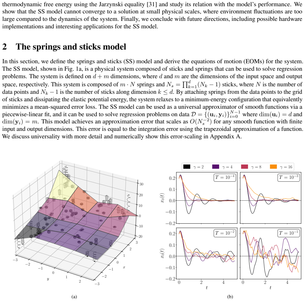
The machinery is the springs-and-sticks (SS) model itself: a grid of jointed sticks whose endpoint coordinates x_i are the parameters, with stick kinetic energy (translational plus rotational) and a spring potential U = (k/2) Σ_j (ŷ(u_j) − y_j)^2 that makes the elastic energy equal the mean-squared-error loss. Dissipation is added via a Langevin thermostat, giving linear stochastic equations dx/dt = ẋ and dẋ/dt = M^{-1} f − γ ẋ + σ ξ̇ with σ = √(2γ T k_b / M), so the bath's temperature and the friction coefficient enter through the fluctuation-dissipation relation. The thermodynamic analysis relies on the Jarzynski equality ΔF = k_b T ln⟨e^{−W/k_b T}⟩ to estimate the free-energy change from
What would settle it
Run the SS system from an initial state equilibrated at temperature T, then measure ΔF via the Jarzynski equality while varying only the friction coefficient γ (or only the speed at which the springs are engaged). If the measured minimum ΔF_min still depends on γ, the quantity is dissipated work along a protocol, not a free-energy barrier—and the TLB as a thermodynamic floor does not hold.
Extended reading notes
Core claim
The central claim is that the springs-and-sticks system is a universal approximator of smooth functions and that its learning obeys a thermodynamic bound. Training is physical relaxation: the mesh's endpoint positions are the trainable parameters, springs implement the squared-error loss, and friction plus thermal noise (a linear Langevin equation) drives the system toward the energy minimum. Using the Jarzynski equality, the authors measure the free energy released during training and find empirically that as the spring constant and mass shrink, the released free energy decreases until it plateaus at a value ΔF_min, the thermodynamic learning barrier. Below that barrier the SS system is una
Load-bearing premise
The quantitative barrier claim rests on identifying the number obtained from the Jarzynski equality, computed from trajectories that start at randomly initialized, non-thermal positions, with a genuine free-energy difference; a true free-energy difference is a state function and would not depend on the protocol or the friction coefficient.
Editorial extensions
If this is right
- If the thermodynamic learning barrier is real, any physical learning machine of a given parameter count operating in a bath at temperature T with friction γ must release at least ΔF_min ∝ k_b T γ during training; hardware that dissipates less cannot converge.
- The scaling ΔF_min ∝ N_s ties model expressivity to energetic cost, implying an explicit energy–accuracy tradeoff for the SS model: approximation error E = O(N_s^{-2}) with E = O(ΔF_min^{-2}).
- The barrier gives a design rule for thermodynamic or physical neural hardware: the effective spring constant of the parameters must be large compared to k_b T, or thermal fluctuations wash out learning.
- If the authors' conjecture generalizes, every learning algorithm implemented in a physical substrate has a minimum free-energy cost set by its phase-space volume and environment, making energy benchmarking of learning machines possible.
- The SS model's regression performance comparable to single-layer MLPs suggests that physical relaxation can serve as an alternative training mechanism without backpropagation.
Reading between the lines
- The dependence of the measured free-energy change on the friction coefficient γ suggests that what is being measured is protocol-dependent dissipated work rather than a state-function free energy; a decisive test would initialize the system at thermal equilibrium and see whether the plateau persists.
- Because the SS dynamics are linear, the barrier can likely be derived exactly from the entropy-production formulas rather than simulated, converting an empirical observation into a testable analytic bound.
- The equivalence between a variable-length SS mesh and a one-hidden-layer ReLU network suggests the TLB could be measured on standard neural-network parameter spaces, testing whether the barrier is substrate-specific or a general property of learning dynamics.
- The reported E = O(ΔF_min^{-2}) relation is a concrete prediction that could be checked against neural scaling-law exponents if 'compute' is measured in dissipated free energy rather than FLOPs.
Editorial analysis
A structured set of objections, weighed in public.
Referee Report
Summary. The paper introduces a mechanical 'springs and sticks' (SS) model for regression. A grid of connected rigid sticks is coupled to data points by springs; the potential energy encodes a mean-squared-error loss, and damped Langevin dynamics drive the system to a low-energy configuration. The authors derive the Lagrangian and equations of motion, prove an O(N_s^{-2}) piecewise-linear approximation error, and show numerically that the model performs comparably to single-layer MLPs on small regression tasks. The paper's main advertised result is a 'thermodynamic learning barrier' (TLB): a minimum free-energy change ΔF_min that the system must release in order to learn, claimed to scale as the number of sticks N_s, the temperature T, and the friction coefficient γ.
Significance. If the thermodynamic claim were sound, it would provide a physically motivated, quantitative floor on the energy required for a mechanical learning system, with potential implications for energy-efficient hardware and for connections between learning and thermodynamics. The paper has real strengths: the linear Lagrangian and Langevin formulation are explicit, the universal-approximation error bound in Appendix A is concrete, the regression experiments are reproducible in structure, and the authors provide public code. These parts of the paper are credible. However, the central thermodynamic result rests on an invalid use of the Jarzynski equality, and the reported scaling laws are not supported by a genuine free-energy calculation. The paper's novelty is substantially contained in the TLB claim, so the thermodynamic contribution needs major revision.
major comments (4)
- [§3.2, Eq. (6)] The Jarzynski equality is applied to compute ΔF from trajectories whose initial conditions are described as 'randomly initialized.' The equality is valid only when the initial ensemble is the canonical (Boltzmann) distribution for the initial Hamiltonian. No thermalization step, equilibrium sampling procedure, or trajectory count is reported. For this quadratic system an exact Gaussian free-energy calculation is available; alternatively, initial conditions should be drawn from the Boltzmann distribution. As written, the quantity in Eq. (6) is not established to be a free-energy difference.
- [§3.2, Fig. 4b] The reported scaling ΔF_min ∝ k_B T γ is incompatible with the interpretation of ΔF as an equilibrium free-energy difference. A free energy is a state function and cannot depend on the friction coefficient γ or on the relaxation protocol. The observed γ dependence is the signature of protocol-dependent dissipated work, not free energy. Consequently, the 'thermodynamic learning barrier' as a minimum free energy required for learning is unsecured. The authors need either to compute the true equilibrium free-energy difference (possible in closed form for a Gaussian potential) or to reframe the claim in terms of dissipated work, which would not support the stated barrier interpretation.
- [§3.2, Figs. 3–4a] The TLB is identified from the same scale sweep in which the average loss is observed to increase sharply, so the correlation between rising loss and falling ΔF is partly by construction. The criterion for 'cannot learn' and the rule for reading off the plateau value ΔF_min are not defined, and no error bars or independent-trajectory statistics are reported. An objective threshold and uncertainty quantification are needed before the scaling laws ΔF_min ∝ N_s, T, γ can be assessed.
- [§3.2, last paragraph; Appendix A] The claimed power law E = O(ΔF_min^{-2}) is not an independent empirical scaling law. It is obtained by substituting the approximation bound E = O(N_s^{-2}) from Appendix A into the fitted relation ΔF_min ∝ N_s from Fig. 4a. Because the fit and the interpretation of ΔF_min as a free energy are themselves unsecured, this relation should be removed or replaced by direct measurements of E as a function of ΔF_min over independent parameter sweeps.
minor comments (5)
- [§3.2] Typo: 'uncapable' should be 'incapable.'
- [§2.1] The notation N_s = Q_{k=1}^d (N_k − 1) is typeset awkwardly; please clarify that it is a product over dimensions.
- [§2.2] The text states that for k > 0 and M = 0 the system becomes an Ornstein–Uhlenbeck process, but the model is defined with nonzero mass. The overdamped limit should be derived explicitly or stated as a limit.
- [Appendix A] The abstract and Section 1 claim universal approximation of continuous functions, but the error bound assumes a bounded Hessian. Please state the smoothness assumption consistently.
- [Eq. (6)] The sign convention ΔF = F_i − F_f is nonstandard and easily confused with the usual Jarzynski convention. A one-line clarification that this is the negative of the conventional free-energy change would help.
Circularity Check
No significant circularity: the TLB scalings are empirical observations, not fitted re-predictions; the core derivations are self-contained.
full rationale
The paper's central derivation chain is self-contained. The SS Lagrangian and EOMs are derived from first principles (Eq. 2, Appendix C); universality and the O(N_s^{-2}) approximation error are established in Appendix A via the trapezoidal rule; and the regression comparison with MLPs is an external empirical benchmark. The thermodynamic learning barrier is an observed phenomenon: Eq. (6) is Jarzynski's equality, and ΔF is computed from simulated trajectories and plotted against the average loss as a function of k; no parameter is fitted to the quantity it later predicts. The scaling E = O(ΔF_min^{-2}) is an algebraic consequence of the independently established E = O(N_s^{-2}) and the empirically observed ΔF_min ∝ N_s, not a circular fit. The claims ΔF_min ∝ N_s and ΔF_min ∝ k_B T γ are likewise presented as empirical findings from Figs. 4a and 4b, not as predictions derived from fitted inputs. The paper cites affiliated prior work only in passing (thermodynamic hardware [20,21]) and does not rest any load-bearing argument on a self-citation. A legitimate physics concern is that Eq. (6) is applied to non-equilibrium initial conditions, so the measured quantity may be dissipated work rather than a true free energy; however, that is a correctness/interpretation issue, not circularity by construction, and per the rules it is not scored here.
Assumptions & free parameters
free parameters (4)
- Learning-barrier threshold =
not quantified
- Scale sweep k = |M| =
1e-31 to 1e-13 (Fig. 3)
- Simulation hyperparameters =
Δt=0.1, two Euler-Maruyama steps per epoch, batch size 16, epochs=9, 4x4 stick grid, MLP width 16
- Temperature and friction ranges =
T from 1e-3 to 1e2, γ from 0.1 to 1e2
assumptions (5)
- ad hoc to paper The initial sticks configuration is a valid starting point for the Jarzynski free energy estimate (an equilibrium distribution is implicitly assumed).
- domain assumption The Langevin thermostat with scalar temperature T and friction γ follows the fluctuation-dissipation relation σ = sqrt(2γ T k_b / M).
- standard math Piecewise-linear interpolation on a tensor grid achieves error O(N^{-2}) (per dimension) for functions with bounded Hessian.
- domain assumption Stick extrema are fixed in the input coordinates and move only in the output coordinates, with fixed lattice spacing.
- ad hoc to paper The TLB phenomenon and its scalings transfer from this linear mechanical system to other learning machines and to neural scaling laws.
invented entities (1)
-
Thermodynamic learning barrier (TLB)
Cite this review
Pith. "Pith review of Learning with springs and sticks." pith.science (2026). https://pith.science/paper/WM4FG5YL
@misc{pith2026250819015,
  author       = {Pith},
  title        = {Pith review of: Learning with springs and sticks},
  year         = {2026},
  howpublished = {\url{https://pith.science/paper/WM4FG5YL}},
  note         = {Machine review of arXiv:2508.19015}
}
read the original abstract
Learning is a physical process. Here, we aim to study a simple dynamical system composed of springs and sticks capable of arbitrarily approximating any continuous function. The main idea of our work is to use the sticks to mimic a piecewise-linear approximation of the given function, use the potential energy of springs to encode a desired mean squared error loss function, and converge to a minimum-energy configuration via dissipation. We apply the proposed simulation system to regression tasks and show that its performance is comparable to that of multi-layer perceptrons. In addition, we study the thermodynamic properties of the system and find a relation between the free energy change of the system and its ability to learn an underlying data distribution. We empirically find a \emph{thermodynamic learning barrier} for the system caused by the fluctuations of the environment, whereby the system cannot learn if its change in free energy hits such a barrier. We believe this simple model can help us better understand learning systems from a physical point of view.
Figures


Figures from the paper (3 more)


Reference graph
Works this paper leans on
-
[49]
Entropy production in linear Langevin systems
Gabriel T Landi, Tânia Tomé, and Mário J De Oliveira. “Entropy production in linear Langevin systems”. In:Journal of Physics A: Mathematical and Theoretical 46.39 (2013), p. 395001
work page 2013
-
[1]
Quantifying the Carbon Emissions of Machine Learning
Alexandre Lacoste et al. Quantifying the Carbon Emissions of Machine Learning . 2019. arXiv: 1910.09700 [cs.CY]. URL: https://arxiv.org/abs/1910.09700
arXiv 2019
-
[2]
Energy and Policy Considerations for Deep Learning in NLP
Emma Strubell, Ananya Ganesh, and Andrew McCallum. Energy and Policy Considerations for Deep Learning in NLP. 2019. arXiv: 1906.02243 [cs.CL]
arXiv 2019
-
[3]
LLMCarbon: Modeling the End-to-End Carbon Footprint of Large Language Models
Ahmad Faiz et al. “LLMCarbon: Modeling the End-to-End Carbon Footprint of Large Language Models”. In: The Twelfth International Conference on Learning Representations . 2024. URL: https://openreview.net/ forum?id=aIok3ZD9to
work page 2024
-
[4]
Deep Unsupervised Learning using Nonequilibrium Thermodynamics
Jascha Sohl-Dickstein et al. Deep Unsupervised Learning using Nonequilibrium Thermodynamics. 2015. arXiv: 1503.03585 [cs.LG]. URL: https://arxiv.org/abs/1503.03585
arXiv 2015
-
[5]
Denoising Diffusion Probabilistic Models
Jonathan Ho, Ajay Jain, and Pieter Abbeel. Denoising Diffusion Probabilistic Models. 2020. arXiv: 2006.11239 [cs.LG]. URL: https://arxiv.org/abs/2006.11239
arXiv 2020
-
[6]
Neural networks and physical systems with emergent collective computational abilities
John J Hopfield. “Neural networks and physical systems with emergent collective computational abilities.” In: Proceedings of the national academy of sciences 79.8 (1982), pp. 2554–2558
1982
-
[7]
A learning algorithm for Boltzmann machines
David H Ackley, Geoffrey E Hinton, and Terrence J Sejnowski. “A learning algorithm for Boltzmann machines”. In: Cognitive science 9.1 (1985), pp. 147–169
work page 1985
Show all 64 references
-
[8]
A fast learning algorithm for deep belief nets
Geoffrey E Hinton, Simon Osindero, and Yee-Whye Teh. “A fast learning algorithm for deep belief nets”. In:Neural computation 18.7 (2006), pp. 1527–1554
2006
-
[9]
A tutorial on energy-based learning
Yann LeCun et al. “A tutorial on energy-based learning”. In: Predicting structured data 1.0 (2006)
2006
-
[10]
GenPhys: From Physical Processes to Generative Models
Ziming Liu et al. GenPhys: From Physical Processes to Generative Models. 2023. arXiv: 2304.02637 [cs.LG]. URL: https://arxiv.org/abs/2304.02637
2023 arXiv
-
[11]
Neural Thermodynamic Integration: Free Energies from Energy- Based Diffusion Models
Bálint Máté, François Fleuret, and Tristan Bereau. “Neural Thermodynamic Integration: Free Energies from Energy- Based Diffusion Models”. In: The Journal of Physical Chemistry Letters 15.45 (2024), pp. 11395–11404. 7
2024
-
[12]
adaline
Bernard Widrow et al. Adaptive" adaline" Neuron Using Chemical" memistors.". 1960
1960
-
[13]
“Neural” computation of decisions in optimization problems
John J Hopfield and David W Tank. ““Neural” computation of decisions in optimization problems”. In:Biological cybernetics 52.3 (1985), pp. 141–152
1985
-
[14]
Neuromorphic electronic systems
Carver Mead. “Neuromorphic electronic systems”. In: Proceedings of the IEEE 78.10 (1990), pp. 1629–1636
1990
-
[15]
A survey of neuromorphic computing and neural networks in hardware
Catherine D Schuman et al. “A survey of neuromorphic computing and neural networks in hardware”. In: arXiv preprint arXiv:1705.06963 (2017)
2017 arXiv
-
[16]
Memristive crossbar arrays for brain-inspired computing
Qiangfei Xia and J Joshua Yang. “Memristive crossbar arrays for brain-inspired computing”. In:Nature materials 18.4 (2019), pp. 309–323
2019
-
[17]
Deep physical neural networks trained with backpropagation
Logan G Wright et al. “Deep physical neural networks trained with backpropagation”. In: Nature 601.7894 (2022), pp. 549–555
2022
-
[18]
Photonic machine learning with on-chip diffractive optics
Tingzhao Fu et al. “Photonic machine learning with on-chip diffractive optics”. In:Nature Communications 14.1 (2023), p. 70
2023
-
[19]
Training of Physical Neural Networks
Ali Momeni et al. Training of Physical Neural Networks. 2024. arXiv: 2406.03372 [physics.app-ph]. URL: https://arxiv.org/abs/2406.03372
2024 arXiv
-
[20]
Coles et al
Patrick J. Coles et al. Thermodynamic AI and the fluctuation frontier. 2023. arXiv: 2302.06584 [cs.ET]
2023 arXiv
-
[21]
Thermodynamic Computing System for AI Applications
Denis Melanson et al. Thermodynamic Computing System for AI Applications . 2023. arXiv: 2312 . 04836 [cs.ET]. URL: https://arxiv.org/abs/2312.04836
2023 arXiv
-
[22]
Analog VLSI implementation of neural systems
Carver Mead and Mohammed Ismail. Analog VLSI implementation of neural systems. V ol. 80. Springer Science & Business Media, 2012
2012
-
[23]
An artificial spiking quantum neuron
Lasse Bjørn Kristensen et al. “An artificial spiking quantum neuron”. In: npj Quantum Information 7.1 (2021), p. 59
2021
-
[24]
Nanosecond protonic programmable resistors for analog deep learning
Murat Onen et al. “Nanosecond protonic programmable resistors for analog deep learning”. In: Science 377.6605 (2022), pp. 539–543
2022
-
[25]
The mathematical mechanic: using physical reasoning to solve problems
Mark Levi. “The mathematical mechanic: using physical reasoning to solve problems”. In: (2023)
2023
-
[26]
Least Squares as Springs
Joshua Loftus. Least Squares as Springs. New York University. Feb. 2022. URL: https://joshualoftus. com/posts/2020-11-23-least-squares-as-springs/least-squares-as-springs.html
2022
-
[27]
Optimization by simulated annealing
Scott Kirkpatrick, C Daniel Gelatt Jr, and Mario P Vecchi. “Optimization by simulated annealing”. In: science 220.4598 (1983), pp. 671–680
1983
-
[28]
A quantum adiabatic evolution algorithm applied to random instances of an NP-complete problem
Edward Farhi et al. “A quantum adiabatic evolution algorithm applied to random instances of an NP-complete problem”. In: Science 292.5516 (2001), pp. 472–475
2001
-
[29]
Environment-assisted quantum transport
Patrick Rebentrost et al. “Environment-assisted quantum transport”. In: New Journal of Physics 11.3 (2009), p. 033003
2009
-
[30]
Adiabatic quantum computation
Tameem Albash and Daniel A Lidar. “Adiabatic quantum computation”. In: Reviews of Modern Physics 90.1 (2018), p. 015002
2018
-
[31]
Nonequilibrium equality for free energy differences
Christopher Jarzynski. “Nonequilibrium equality for free energy differences”. In: Physical Review Letters 78.14 (1997), p. 2690
1997
-
[32]
Mathematical methods of classical mechanics
Vladimir Igorevich Arnol’d. Mathematical methods of classical mechanics. V ol. 60. Springer Science & Business Media, 2013
2013
-
[33]
Adaptive mixtures of local experts
Robert A Jacobs et al. “Adaptive mixtures of local experts”. In: Neural computation 3.1 (1991), pp. 79–87
1991
-
[34]
Sparse grids
Hans-Joachim Bungartz and Michael Griebel. “Sparse grids”. In: Acta numerica 13 (2004), pp. 147–269
2004
-
[35]
Introduction to algorithms
Thomas H Cormen et al. Introduction to algorithms. MIT press, 2022
2022
-
[36]
Irreversibility and generalized noise
Herbert B Callen and Theodore A Welton. “Irreversibility and generalized noise”. In: Physical Review 83.1 (1951), p. 34
1951
-
[37]
Statistical-mechanical theory of irreversible processes. I. General theory and simple applications to magnetic and conduction problems
Ryogo Kubo. “Statistical-mechanical theory of irreversible processes. I. General theory and simple applications to magnetic and conduction problems”. In: Journal of the physical society of Japan 12.6 (1957), pp. 570–586
1957
-
[38]
Stochastic thermodynamics, fluctuation theorems and molecular machines
Udo Seifert. “Stochastic thermodynamics, fluctuation theorems and molecular machines”. In: Reports on progress in physics 75.12 (2012), p. 126001
2012
-
[39]
Energy spectrum of a Langevin oscillator
Y Mishin and J Hickman. “Energy spectrum of a Langevin oscillator”. In: Physical Review E 94.6 (2016), p. 062151. 8
2016
-
[40]
Stochastic Thermodynamics: An Introduction
Luca Peliti and Simone Pigolotti. Stochastic Thermodynamics: An Introduction. Princeton University Press, 2021
2021
-
[41]
A stochastic approximation method
Herbert Robbins and Sutton Monro. “A stochastic approximation method”. In: The annals of mathematical statistics (1951), pp. 400–407
1951
-
[42]
Curtis, and Jorge Nocedal
Léon Bottou, Frank E. Curtis, and Jorge Nocedal. Optimization Methods for Large-Scale Machine Learning. 2018. arXiv: 1606.04838 [stat.ML]. URL: https://arxiv.org/abs/1606.04838
2018 arXiv
-
[43]
Continuous time analysis of momentum methods
Nikola B Kovachki and Andrew M Stuart. “Continuous time analysis of momentum methods”. In: Journal of Machine Learning Research 22.17 (2021), pp. 1–40
2021
-
[44]
Stochastic differential equations
Philip E Protter. Stochastic differential equations. Springer, 2005
2005
-
[45]
Brownian motion and stochastic calculus
Ioannis Karatzas and Steven Shreve. Brownian motion and stochastic calculus. V ol. 113. springer, 2014
2014
-
[46]
Scalable gradients for stochastic differential equations
Xuechen Li et al. “Scalable gradients for stochastic differential equations”. In: International Conference on Artificial Intelligence and Statistics (2020)
2020
-
[47]
Kai Wang et al.Neural Network Diffusion. 2024. arXiv: 2402.13144 [cs.LG]. URL: https://arxiv.org/ abs/2402.13144
2024 arXiv
-
[48]
Entropy production in full phase space for continuous stochastic dynamics
Richard E Spinney and Ian J Ford. “Entropy production in full phase space for continuous stochastic dynamics”. In: Physical Review E 85.5 (2012), p. 051113
2012
-
[50]
Speed Limits for Deep Learning
Inbar Seroussi et al. “Speed Limits for Deep Learning”. In: arXiv preprint arXiv:2307.14653 (2023)
2023 arXiv
-
[51]
Irreversibility and heat generation in the computing process
Rolf Landauer. “Irreversibility and heat generation in the computing process”. In: IBM journal of research and development 5.3 (1961), pp. 183–191
1961
-
[52]
The thermodynamics of computation—a review
Charles H Bennett. “The thermodynamics of computation—a review”. In: International Journal of Theoretical Physics 21 (1982), pp. 905–940
1982
-
[53]
Notes on Landauer’s principle, reversible computation, and Maxwell’s Demon
Charles H Bennett. “Notes on Landauer’s principle, reversible computation, and Maxwell’s Demon”. In:Studies In History and Philosophy of Science Part B: Studies In History and Philosophy of Modern Physics 34.3 (2003), pp. 501–510
2003
-
[54]
Stochastic thermodynamics of learning
Sebastian Goldt and Udo Seifert. “Stochastic thermodynamics of learning”. In: Physical review letters 118.1 (2017), p. 010601
2017
-
[55]
Deep learning scaling is predictable, empirically
Joel Hestness et al. “Deep learning scaling is predictable, empirically”. In: arXiv preprint arXiv:1712.00409 (2017)
2017 arXiv
-
[56]
Scaling laws for neural language models
Jared Kaplan et al. “Scaling laws for neural language models”. In: arXiv preprint arXiv:2001.08361 (2020)
2001 arXiv
-
[57]
Explaining neural scaling laws
Yasaman Bahri et al. “Explaining neural scaling laws”. In: Proceedings of the National Academy of Sciences 121.27 (2024), e2311878121
2024
-
[58]
Lagrangian for RLC circuits using analogy with the classical mechanics concepts
Albertus Hariwangsa Panuluh and Asan Damanik. “Lagrangian for RLC circuits using analogy with the classical mechanics concepts”. In: Journal of Physics: Conference Series. V ol. 909. 1. IOP Publishing. 2017, p. 012005
2017
-
[59]
Exponential quantum speedup in simulating coupled classical oscillators
Ryan Babbush et al. “Exponential quantum speedup in simulating coupled classical oscillators”. In: Physical Review X 13.4 (2023), p. 041041
2023
-
[60]
High-order quantum algorithm for solving linear differential equations
Dominic W Berry. “High-order quantum algorithm for solving linear differential equations”. In: Journal of Physics A: Mathematical and Theoretical 47.10 (2014), p. 105301
2014
-
[61]
Quantum Algorithm for Systems of Linear Equa- tions with Exponentially Improved Dependence on Precision
Andrew M. Childs, Robin Kothari, and Rolando D. Somma. “Quantum Algorithm for Systems of Linear Equa- tions with Exponentially Improved Dependence on Precision”. In: SIAM Journal on Computing 46.6 (Jan. 2017), pp. 1920–1950. ISSN : 1095-7111. DOI: 10.1137/16m1087072. URL: http...
2017 doi
-
[62]
Quantum algorithm for linear differential equations with exponentially improved dependence on precision
Dominic W Berry et al. “Quantum algorithm for linear differential equations with exponentially improved dependence on precision”. In: Communications in Mathematical Physics 356 (2017), pp. 1057–1081
2017
-
[63]
Further improving quantum algorithms for nonlinear differential equations via higher-order methods and rescaling
Pedro Costa et al. “Further improving quantum algorithms for nonlinear differential equations via higher-order methods and rescaling”. In: arXiv preprint arXiv:2312.09518 (2023)
2023 arXiv
-
[64]
Fast quantum algorithm for differential equations
Mohsen Bagherimehrab et al. “Fast quantum algorithm for differential equations”. In:arXiv preprint arXiv:2306.11802 (2023). 9 Supplementary Material A Universal approximation The springs and sticks system is a universal approximator of continuous functions with bounded Hessian...
2023
Reviewed August 5, 2026 · model on record in the stance chip above.
Discussion (0). Sign in to comment.