REVIEW 3 major objections 4 minor 34 references
Variational Bayes on Manifolds
T0 review · 3 major / 4 minor · reviewed 2026-08-14 · deepseek-v4-flash
Pith's one-line read Variational Bayes can be run directly on curved parameter spaces, with proven convergence to a local mode of the evidence lower bound.
desk verdict Solid framework for natural-gradient VB on manifolds, but the advertised O(1/T^{2−2ε}) rate for strongly retraction-convex ELBOs doesn't follow from the proof. read the letter →
The pith
A machine-rendered reading of the paper's core claim, the machinery that carries it, and where it could break.
The reading
What carries the argument
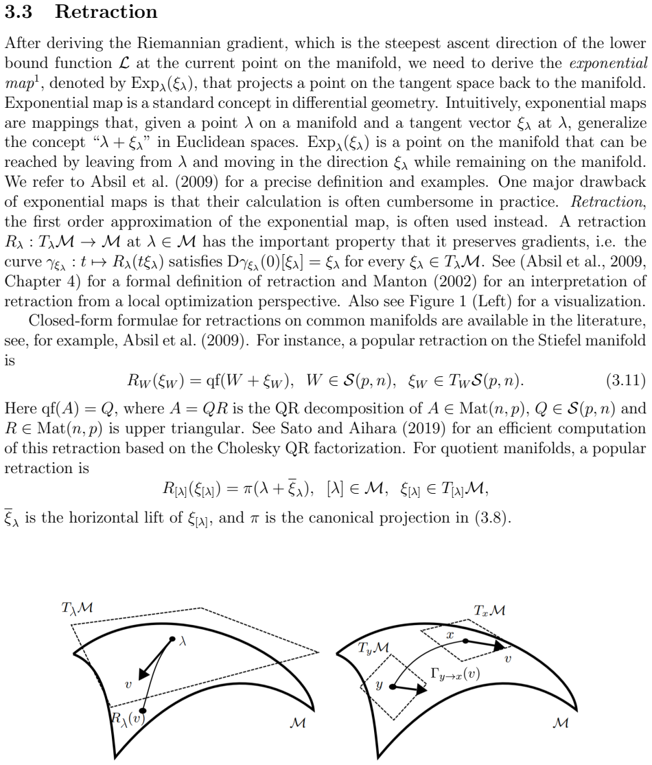
The central object is the variational family $\mathcal{N}=\{q_\lambda\}$ viewed as a Riemannian submanifold or quotient manifold of the parameter space, equipped with the Fisher-Rao metric $\langle\zeta,\xi\rangle=\zeta^\top I_F(\lambda)\xi$. Lemma 3.1 identifies the natural gradient $I_F(\lambda)^{-1}\nabla L(\lambda)$ with the Riemannian gradient of the lower bound in the ambient manifold; for submanifolds it is projected onto the tangent space, and for quotient manifolds its horizontal lift is the Riemannian gradient. The update uses a retraction $R_\lambda$, a first-order approximation of the exponential map that replaces the Euclidean move $\lambda+\xi$, and a vector transport that pushes momentum vectors between tangent spaces. Theorem 1 provides the convergence machinery: bounded gradients with martingale-difference noise, retraction-Lipschitz gradients, and, for the faster rate, strong retraction-convexity.
What would settle it
Run the Manifold Gaussian VB algorithm on a low-dimensional problem where the exact Fisher information $I_F(\Sigma)$ is computable, compare the exact natural gradient with the approximation $(\Sigma\otimes\Sigma)\nabla_\Sigma L$, and test whether the approximate update still drives $\mathbb{E}|\nabla L|^2$ to zero at the claimed rate; a measured bias that does not shrink with step size, or divergence for some initialization, would falsify the claim that the practical algorithm inherits Theorem 1's guarantees.
Extended reading notes
Core claim
The central claim is that constrained variational inference is not a special case to be patched with factorizations, but a genuine Riemannian optimization problem. Lemma 3.1 shows that the natural gradient $I_F(\lambda)^{-1}\nabla L(\lambda)$ is the Riemannian gradient of the lower bound when the manifold is equipped with the Fisher-Rao metric, so the steepest-ascent direction automatically respects the information geometry of the variational family. Algorithm 1 iterates $\lambda_{t+1}=R_{\lambda_t}(\epsilon Y_t)$, with $Y_t$ a momentum-averaged estimate of the projected natural gradient; for submanifolds the projection is orthogonal, and for quotient manifolds it is the horizontal lift. Theorem 1 states that with step size $1/\sqrt{T}$ the squared Riemannian gradient norm is driven below $C/\sqrt{T}$, and that strong retraction-convexity improves the expected squared distance to the optimum to $O(T^{2\epsilon-2})$. The Gaussian instantiation uses the full covariance matrix on the manifold of symmetric positive-definite matrices with the approximation $I_F(\Sigma)\approx\Sigma^{-1}\otimes\Sigma^{-1}$, and the Wishart instantiation uses analogous natural-gradient preconditioning; both are tested on data where they converge faster and more stably than previous VB methods.
Load-bearing premise
The practical algorithms inherit the paper's convergence rates only if the approximate natural-gradient formulas are close enough to the true natural gradient; the paper gives no error bound for these approximations.
Editorial extensions
If this is right
- For a non-convex evidence lower bound, running the manifold VB algorithm for $T$ steps with step size $1/\sqrt{T}$ gives $\min_{t\le T}\mathbb{E}|\nabla L(\lambda_t)|^2\le C/\sqrt{T}$.
- For a strongly retraction-convex ELBO, choosing step size $1/T^\epsilon$ yields $\mathbb{E}(\lambda_T-\lambda^*)^2\le C_\epsilon T^{2\epsilon-2}$, approaching $O(1/T^2)$ as $\epsilon$ tends to zero.
- Because the natural gradient is parameterization-invariant, the manifold update is the same geometric object regardless of how the variational family is parameterized.
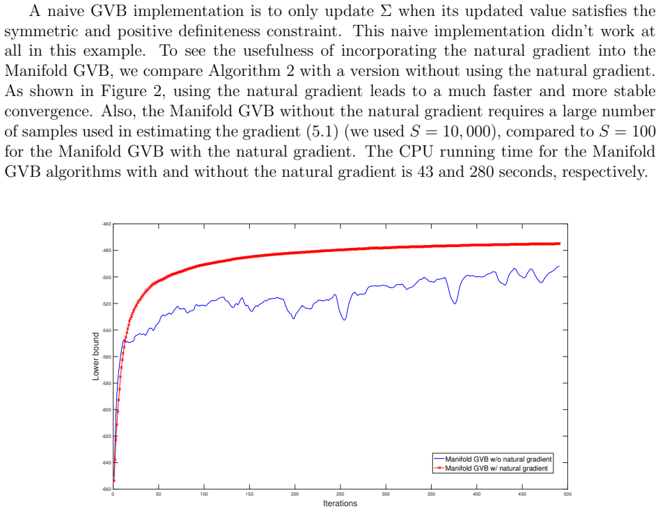
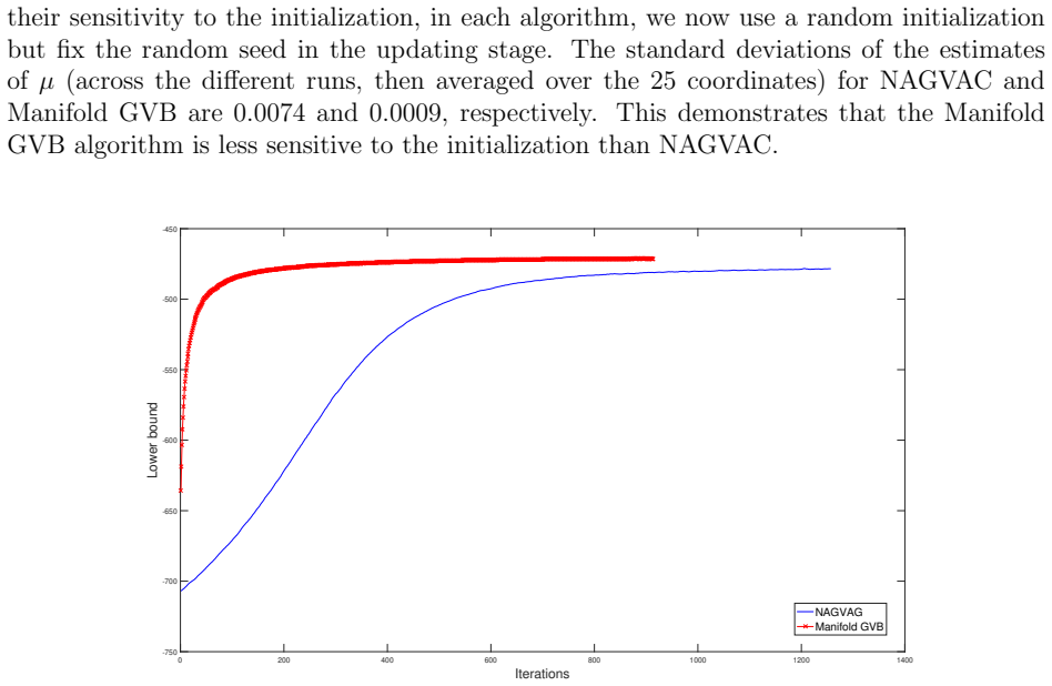
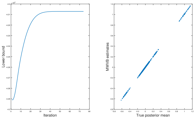
- Gaussian variational Bayes can use full covariance matrices on the positive-definite manifold rather than factorized covariance structures, with faster convergence and lower variance across random initializations than a factorized Gaussian VB.
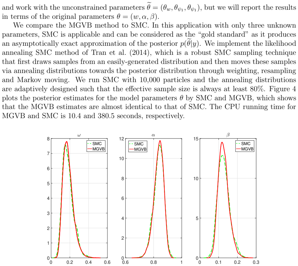
- The Wishart instantiation matches a gold-standard sequential Monte Carlo posterior estimate for a financial GARCH model while using a small fraction of the compute time.
Reading between the lines
- Editorial inference: the convergence rates are proved for the exact Riemannian gradient, so an error analysis for the approximate natural gradients, such as $\Sigma^{-1}\otimes\Sigma^{-1}$ in the Gaussian case, would turn the practical algorithms into theorems; until then, the rates are safest read as applying to the idealized update.
- Editorial inference: the same template, projecting a natural-gradient direction onto the tangent space and retracting, should transfer to other constrained variational families, such as low-rank factor covariances or positive-definite matrices in Gaussian processes, wherever a retraction and vector transport exist.
- Editorial inference: a direct comparison of updates using the exact Fisher information matrix against the $\Sigma^{-1}\otimes\Sigma^{-1}$ approximation on low-dimensional Gaussian VB would give a testable measure of how much of the observed speedup comes from the approximation rather than from the manifold geometry.
Signed reviews
Editorial analysis
A structured set of objections, weighed in public.
Referee Report
Summary. The paper proposes a manifold-based variational Bayes framework. It treats the variational parameter space as a Riemannian manifold, equips it with the Fisher-Rao metric, identifies the natural gradient with the Riemannian gradient (Lemma 3.1), handles submanifold and quotient cases, and runs Riemannian SGD with momentum. It states convergence rates of order O(1/sqrt(T)) for non-convex ELBOs and O(1/T^(2-2ε)) for strongly retraction-convex ELBOs. It then instantiates Manifold Gaussian VB and Manifold Wishart VB, with numerical experiments on logistic regression, GARCH volatility, and covariance estimation, plus comparisons to NAGVAC and SMC.
Significance. If the convergence theorem were correct, this would be a valuable generalization of variational Bayes to constrained parameter spaces, combining information-geometric preconditioning with Riemannian optimization. The geometric derivations in Lemmas 3.1 and 3.2 are clean and self-contained, the algorithmic descriptions are concrete, and the authors provide code and an SMC comparison. However, the advertised fast strongly-convex rate is not supported by the proof as written, and the implemented algorithms rely on unquantified approximations that the theorem does not cover. These issues affect the paper's central guarantees, so the significance is currently conditional on a repair of the proof and a clarification of the scope of the theoretical claims.
major comments (3)
- [Section 4, proof of Theorem 1(ii), around Eq. (6.27)] The proof sets rho = 1 - gamma/(4*mu_tilde*(1-zeta)) immediately before Eq. (6.22), so 1-rho = O(gamma). The unrolled recursion then gives EV_T <= rho^T C0 + C*gamma^2/(1-rho), but the next line replaces C*gamma^2/(1-rho) by C*gamma^2. This is algebraically false: C*gamma^2/(1-rho) = 4*C*mu_tilde*(1-zeta)*gamma = O(gamma). With gamma = T^{-epsilon}, the correct noise floor is O(T^{-epsilon}), not O(T^(2*epsilon-2)). A second inconsistency appears in the same paragraph: gamma^2 = T^(-2*epsilon) equals T^(2*epsilon-2) only when epsilon = 1/2. Thus the advertised rate O(1/T^(2-2*epsilon)) in the abstract and Theorem 1 is unsupported by the proof as written.
- [Section 5.1, Eqs. (5.2)-(5.4), and Section 5.2, Eqs. (5.7)-(5.8)] The convergence theorem is proved for exact Riemannian gradients with unbiased estimators. The implemented Manifold Gaussian VB uses the approximation IF(Sigma) approx Sigma^{-1} tensor Sigma^{-1}, and the Manifold Wishart VB uses the natural-gradient-like replacements in (5.7) and (5.8). No error bound or perturbation analysis relates these approximate updates to the exact Riemannian gradient required by Theorem 1. Consequently, the stated convergence guarantees do not apply to the algorithms whose numerical behavior is reported. The paper should either prove that these approximations satisfy the theorem's conditions up to controlled errors, or explicitly state that the numerical results are heuristic demonstrations.
- [Section 3.2, Remark 3.1] The quotient-manifold construction defines the horizontal space as the orthogonal complement under the Fisher-Rao metric, but the metric is not invariant along equivalence classes, as Remark 3.1 concedes. The claim that equation (3.10) is independent of the representative lambda in [lambda] is asserted rather than proved. Without metric invariance, the horizontal lift and the induced inner product on the quotient manifold are generally representative-dependent, and the usual Riemannian-submersion condition is exactly what is needed to rule this out. This is a gap in the claimed general framework for quotient manifolds, although the paper's numerical experiments do not depend on this part.
minor comments (4)
- [Abstract] The abstract names Manifold Neural Net VB as one of the two developed algorithms, but the paper actually develops Manifold Gaussian VB and Manifold Wishart VB; the abstract should be corrected to match the body.
- [Figure 3] The legend in Figure 3 reads NAGVAG instead of NAGVAC.
- [Section 4, end of proof of Theorem 1(ii)] The theorem statement bounds E(lambda_T - lambda_*)^2, but the proof bounds E(L(lambda_T) - L(lambda_*)) and E|grad L|^2; the strong-convexity inequality linking squared retraction distance to the function suboptimality is not stated, so the final line of the proof does not directly deliver the theorem's claim.
- [Section 5.1, Eq. (5.2)] The sentence 'One can derive that IF(Sigma) approx Sigma^{-1} tensor Sigma^{-1}' gives no derivation or citation for the approximation; since this approximation is used in the implemented algorithm, a reference or explicit formula would clarify its accuracy.
Circularity Check
No circularity: the manifold VB derivation follows from the Fisher-Rao metric definition and the convergence analysis is an independent extension of prior Riemannian SGD theory; self-citations are not load-bearing.
full rationale
The derivation chain is self-contained. The natural-gradient identity (3.2) and Lemma 3.1 are proved from the definition of the Fisher-Rao metric (3.1), and the projection formulas for submanifolds and quotient manifolds follow from the defining property of a Riemannian gradient; the target conclusions are not used as inputs. Theorem 1 is an extension of the Riemannian SGD analysis in Huang et al. (2015a,b) and Absil et al. (2009), and the proof is carried out in the appendix on the explicit recursion (4.2); the advertised rates are consequences of the proof, not restatements of an assumed bound. The practical approximations in Section 5, such as IF(Σ)≈Σ^{-1}⊗Σ^{-1} in Eq. (5.2), are clearly labeled approximations used to instantiate the algorithm and are not claimed to be derived from Theorem 1; whether they satisfy the theorem's assumptions is a coverage question, not circularity. Self-citations (Tran et al. 2017, 2019, 2021) appear for standard score-function gradient identities and as experimental baselines, and are not load-bearing; the numerical benchmarks also include an analytic inverse-Wishart posterior and an SMC gold standard. The algebraic concern raised about the 1/(1−ρ) term in the strongly retraction-convex rate is a proof-correctness issue, not an equivalence between inputs and outputs, so it does not contribute to the circularity score.
Assumptions & free parameters
free parameters (4)
- Learning rate epsilon
- Momentum weight omega
- Number of Monte Carlo samples S for score-function gradient =
100, 1000, or 10000 in experiments
- Adaptive method hyperparameters for Wishart nu update
assumptions (5)
- domain assumption The variational family {q_lambda} is a smooth Riemannian manifold with the Fisher information matrix IF(lambda) as metric (Section 2, Eq. 2.3).
- domain assumption The score-function gradient estimator is unbiased and has finite variance (Section 4, Eq. 4.2).
- ad hoc to paper The objective satisfies: totally retractive neighborhood of the optimum, L-Lipschitz Riemannian gradient w.r.t. the retraction, and a.s. bounded gradient and noise (Theorem 1).
- ad hoc to paper For quotient manifolds, the Riemannian gradient is well-defined even though the Fisher-Rao metric is not invariant along the equivalence class (Remark 3.1).
- ad hoc to paper The approximate natural gradients used in practice are close enough to the exact Riemannian gradient for the convergence theorem to apply (Eqs. 5.2, 5.7, 5.8).
Cite this review
Pith. "Pith review of Variational Bayes on Manifolds." pith.science (2026). https://pith.science/paper/WOLHUZGI
@misc{pith2026190803097,
  author       = {Pith},
  title        = {Pith review of: Variational Bayes on Manifolds},
  year         = {2026},
  howpublished = {\url{https://pith.science/paper/WOLHUZGI}},
  note         = {Machine review of arXiv:1908.03097}
}
abstract
Variational Bayes (VB) has become a widely-used tool for Bayesian inference in statistics and machine learning. Nonetheless, the development of the existing VB algorithms is so far generally restricted to the case where the variational parameter space is Euclidean, which hinders the potential broad application of VB methods. This paper extends the scope of VB to the case where the variational parameter space is a Riemannian manifold. We develop an efficient manifold-based VB algorithm that exploits both the geometric structure of the constraint parameter space and the information geometry of the manifold of VB approximating probability distributions. Our algorithm is provably convergent and achieves a convergence rate of order $\mathcal O(1/\sqrt{T})$ and $\mathcal O(1/T^{2-2\epsilon})$ for a non-convex evidence lower bound function and a strongly retraction-convex evidence lower bound function, respectively. We develop in particular two manifold VB algorithms, Manifold Gaussian VB and Manifold Neural Net VB, and demonstrate through numerical experiments that the proposed algorithms are stable, less sensitive to initialization and compares favourably to existing VB methods.
Figures
Figures from the paper (2 more)
Reference graph
Works this paper leans on
-
[1]
Absil, P.-A., Mahony, R., and Sepulchre, R. (2009). Optimization algorithms on matrix manifolds . Princeton University Press
work page 2009
-
[2]
Amari, S. (1998). Natural gradient works efficiently in learning. Neural computation , 10(2):251--276
work page 1998
-
[3]
B \'e cigneul, G. and Ganea, O.-E. (2018). Riemannian adaptive optimization methods. arXiv preprint arXiv:1810.00760
arXiv 2018
-
[4]
Berg, R. v. d., Hasenclever, L., Tomczak, J. M., and Welling, M. (2018). Sylvester normalizing flows for variational inference. arXiv preprint arXiv:1803.05649
arXiv 2018
-
[5]
Bollerslev, T. (1986). Generalized autoregressive conditional heteroskedasticity. Journal of Econometrics , 31(3):307 -- 327
work page 1986
-
[6]
Bonnabel, S. (2013). Stochastic gradient descent on Riemannian manifolds. IEEE Transactions on Automatic Control , 58(9):2217--2229
work page 2013
-
[7]
Boumal, N., Mishra, B., Absil, P.-A., and Sepulchre, R. (2014). M anopt, a M atlab toolbox for optimization on manifolds. Journal of Machine Learning Research , 15:1455--1459
work page 2014
-
[8]
Edelman, A., Arias, T., and Smith, A. (1998). The geometry of algorithms with orthogonality constraints. SIAM J. Matrix Anal. Appl. , 20(2):303–353
work page 1998
Show all 34 references
-
[9]
D., Blei, D
Hoffman, M. D., Blei, D. M., Wang, C., and Paisley, J. (2013). Stochastic variational inference. Journal of Machine Learning Research , 14:1303--1347
2013
-
[10]
Huang, W., Absil, P.-A., and Gallivan, K. A. (2015a). A Riemannian symmetric rank-one trust-region method. Mathematical Programming , 150(2):179--216
2015
-
[11]
A., and Absil, P.-A
Huang, W., Gallivan, K. A., and Absil, P.-A. (2015b). A Broyden class of quasi-Newton methods for Riemannian optimization. SIAM Journal on Optimization , 25(3):1660--1685
2015
-
[12]
I., Ghahramani, Z., Jaakkola, T
Jordan, M. I., Ghahramani, Z., Jaakkola, T. S., and Saul, L. K. (1999). An introduction to variational methods for graphical models. Machine learning , 37(2):183--233
1999
-
[13]
Kasai, H., Jawanpuria, P., and Mishra, B. (2019). Adaptive stochastic gradient algorithms on riemannian manifolds. arXiv preprint arXiv:1902.01144
2019 arXiv
-
[14]
Khan, M. E. and Lin, W. (2017). Conjugate-computation variational inference: Converting variational inference in non-conjugate models to inferences in conjugate models. In Proceedings of the 20th International Conference on Artificial Intelligence and Statistics (AISTATS)
2017
-
[15]
Kingma, D. P. and Welling, M. (2013). Auto-encoding variational bayes. arXiv preprint arXiv:1312.6114
2013 arXiv
-
[16]
and Nomizu, K
Kobayashi, S. and Nomizu, K. (1969). Foundations of Differential Geometry, Vols. 1 and 2 . Wiley, New York
1969
-
[17]
Longford, N. T. (1987). A fast scoring algorithm for maximum likelihood estimation in unbalanced mixed models with nested random effects. Biometrika , 74(4):817--827
1987
-
[18]
Manton , J. H. (2002). Optimization algorithms exploiting unitary constraints. IEEE Transactions on Signal Processing , 50(3):635--650
2002
-
[19]
Mardia, K. V. and Marshall, R. J. (1984). Maximum likelihood estimation of models for residual covariance in spatial regression. Biometrika , 71(1):135--146
1984
-
[20]
Martens, J. (2020). New insights and perspectives on the natural gradient method. Journal of Machine Learning Research , 21(146):1--76
2020
-
[21]
M., Nott, D
Ong, V. M., Nott, D. J., Tran, M.-N., Sisson, S. A., and Drovandi, C. C. (2018a). Variational Bayes with synthetic likelihood. Statistics and Computing , 28(4):971--988
2018
-
[22]
M.-H., Nott, D
Ong, V. M.-H., Nott, D. J., and Smith, M. S. (2018b). Gaussian variational approximation with factor covariance structure . Journal of Computational and Graphical Statistics , 27(3):465--478
2018
-
[23]
Rao, C. R. (1945). Information and accuracy attainable in the estimation of statistical parameters. Bull. Calcutta. Math. Soc , 37:81--91
1945
-
[24]
Roy, S. K. and Harandi, M. (2017). Constrained stochastic gradient descent: The good practice. In In Proceedings of the International Conference on Digital Image Computing: Techniques and Applications (DICTA)
2017
-
[25]
and Aihara, K
Sato, H. and Aihara, K. (2019). Cholesky QR-based retraction on the generalized Stiefel manifold . Computational Optimization and Applications , 72(2):293--308
2019
-
[26]
Sato , M. (2001). Online model selection based on the variational bayes. Neural Computation , 13(7):1649--1681
2001
-
[27]
Tagare, H. D. (2011). Notes on optimization on Stiefel manifolds. http://noodle.med.yale.edu/ hdtag/notes/steifel\_notes.pdf
2011
-
[28]
Tran, M.-N., Nguyen, N., Nott, D., and Kohn, R. (2019). Bayesian deep net GLM and GLMM . Journal of Computational and Graphical Statistics
2019
-
[29]
Tran, M.-N., Nguyen, T.-N., and Dao, V.-H. (2021). A practical tutorial on Variational Bayes . arXiv:2103.01327
2021 arXiv
-
[30]
J., and Kohn, R
Tran, M.-N., Nott, D. J., and Kohn, R. (2017). Variational Bayes with intractable likelihood. Journal of Computational and Graphical Statistics , 26(4):873--882
2017
-
[31]
K., and Kohn, R
Tran, M.-N., Pitt, M. K., and Kohn, R. (2014). Annealed important sampling for models with latent variables. http://arxiv.org/abs/1402.6035
2014 arXiv
-
[32]
Tu, L. W. (2011). An introduction to manifolds . Springer New York
2011
-
[33]
Waterhouse, S., MacKay, D., and Robinson, T. (1996). Bayesian methods for mixtures of experts. In Touretzky, M. C. M. D. S. and Hasselmo, M. E., editors, Advances in Neural Information Processing Systems , pages 351--357. MIT Press
1996
-
[34]
Zhou, B., Gao, J., Tran, M.-N., and Gerlach, R. (2020). Manifold optimisation assisted Gaussian variational approximation. Journal of Computational and Graphical Statistics (to appear)
2020
Reviewed August 14, 2026 · model on record in the stance chip above.
Discussion (0). Continue with ORCID to comment.