REVIEW 4 major objections 4 minor 20 references
Two-phase source and reaction coefficient Stefan type problems
T0 review · 4 major / 4 minor · reviewed 2026-08-01 · deepseek-v4-flash
Pith's one-line read Two inverse two-phase Stefan problems are solved by fixed-domain Fourier expansions, recovering time-dependent source and reaction coefficients from Volterra equations and, in the two-boundary case, from Stefan conditions alone.
desk verdict The two-phase extension is real, but the reconstruction is circular and the main theorems are deferred; the central claims don't hold as written. read the letter →
The pith
A machine-rendered reading of the paper's core claim, the machinery that carries it, and where it could break.
The reading
What carries the argument
The machinery is a pair of coordinate transformations ξ_1 = x/s(t), ξ_2 = (x−s(t))/(d−s(t)) that freeze each moving phase onto the fixed interval (0,1), together with the Dirichlet spectral basis φ_n(ξ)=√2 sin(nπξ) (and the mixed Neumann–Dirichlet basis w_n(ξ)=√2 cos((2n−1)πξ/2) for the second problem). Expanding the transformed temperatures in these bases turns the PDEs into ODEs for the spectral coefficients; their explicit solutions, containing exponentials of the time-dependent diffusivities and advection terms, are inserted into the data conditions and differentiated to yield Volterra integral equations of the second kind for the unknown coefficients R_i(t). An exponential substitution
What would settle it
Take a problem with a known, nonconstant R1(t) and compute the spectral coefficient F_1,1(t) of h1 from (5) using the true R1. If F_1,1 contains R1 in its denominator, then substituting the true R1 into the right-hand side of (24) will not reproduce R1 unless the equation is merely an identity; a numerical test with Example 1's setting (where F_1,1 is artificially independent of R1) would not detect this, so a problem with a different f1 that makes the R1-dependence explicit would settle whether (24) is truly a closed-form inversion.
Extended reading notes
Core claim
The central claim is that a two-phase Stefan inverse problem with one moving interface and unknown source coefficients R1(t), R2(t) can be fully solved by (i) subtracting the boundary data, (ii) mapping each moving phase to the unit interval, (iii) expanding in sine eigenfunctions, and (iv) differentiating the overdetermination condition to obtain Volterra equations for R1 and R2 from integral, pointwise, or nonlocal data. For a second problem with two moving interfaces and unknown reaction coefficients P1(t), P2(t), the exponential substitution R_i(t)=exp(−∫_0^t P_i(τ)dτ) converts it into a source-coefficient problem; the two Stefan conditions then determine both auxiliary coefficients simu
Load-bearing premise
The transformed source terms h1 and h2 in Eqs. (5)–(6) are defined through the unknown coefficients R1(t) and R2(t) (they contain 1/R1 and 1/R2 terms), yet the spectral coefficients F_i,n of these terms are treated as known data in the reconstruction formulas (24) and (26); if F_i,n depends on R_i, the claimed explicit linear Volterra structure is not justified.
Editorial extensions
If this is right
- Time-dependent source intensities in a two-phase melting or solidification body can be recovered from a single integral measurement, a single interior point temperature, or a nonlocal weighted average, requiring no interior probes beyond those observations.
- In a two-phase body bounded by two moving fronts, the Stefan energy-balance conditions alone determine both unknown reaction coefficients, removing the need for separate overdetermination measurements.
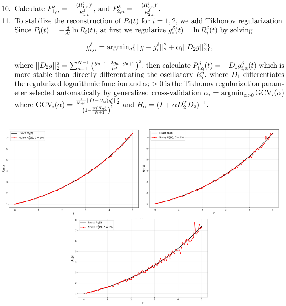
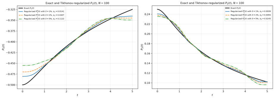
- The explicit spectral-Volterra reconstruction formulas are stable under noisy boundary data once the numerical differentiation step is regularized, as demonstrated at 1%, 2%, and 5% noise levels.
- The existence, uniqueness, and regularity theorems establish that the recovered pairs are genuine weak/strong solutions of the original moving-boundary problem, not merely formal series solutions.
- When only finitely many spectral modes are active, the reconstruction is given in closed form, providing concrete test cases for numerical implementations.
Reading between the lines
- The paper leaves implicit that the reconstruction formulas (24) and (26) are only explicit linear Volterra equations if the transformed source terms h1 and h2 are independent of the sought R1 and R2; when h1 and h2 contain 1/R1 and 1/R2, the equations become nonlinear and the convergence arguments in Lemma 3 and the theorems (which assume bounded, known kernels) would need a separate justification
- The two-boundary result suggests a general counting rule for inverse Stefan problems — the number of recoverable time-dependent coefficients matches the number of independent Stefan conditions — which could guide data requirements in multi-front or multidimensional phase-change problems.
- The numerical instability in the reaction problem is concentrated in the differentiation step P_i = −R_i'/R_i, not in recovering R_i; a testable extension would regularize the logarithmic-derivative estimation directly rather than post-differentiating the reconstructed R_i.
- The regularity assumptions on the data (fourth-order differentiability and strong boundary-compatibility) mean the reconstruction will exhibit smoothing bias when the true temperature lacks such smoothness; quantifying that bias against noise in realistic data would be a natural next step.
Editorial analysis
A structured set of objections, weighed in public.
Referee Report
Summary. The paper studies two inverse Stefan-type problems for heat equations. In the first problem, unknown time-dependent source coefficients R1(t), R2(t) are to be recovered together with the temperature fields in a two-phase one-moving-boundary configuration, using integral, pointwise, or nonlocal overdetermination data. The moving domains are mapped to the fixed interval (0,1), the temperature is expanded in Fourier series of the Dirichlet eigenfunctions, and reconstruction formulas (24), (26), (45), (51) are derived. These formulas are claimed to be Volterra integral equations of the second kind, leading to existence, uniqueness, boundedness, and regularity theorems (Theorems 1–5). In the second problem, a two-moving-boundary configuration with Neumann conditions contains unknown reaction coefficients P1(t),P2(t); via the exponential substitution (67)–(68) it is reduced to an inverse source problem, and the two Stefan conditions are claimed to determine both coefficients without additional overdetermination (Theorem 6, formulas (84)–(85)). Numerical experiments for both examples are discussed.
Significance. If the reconstruction formulas and the accompanying existence, uniqueness, and regularity theorems were correct, the paper would constitute a meaningful extension of the one-phase inverse Stefan analysis of NauKhum (2025) to a genuinely two-phase setting and would support the interesting claim that, in the two-moving-boundary configuration, the two Stefan conditions suffice to determine two time-dependent coefficients. However, the central inversion step is not justified: the spectral coefficients F_i,n fed into the reconstruction formulas are defined through the very unknown coefficients R_i, so the purported Volterra equations are self-referential rather than explicit. The analytical claims are also undermined by the systematic deferral of the key proofs to a self-cited preprint. The numerical examples are carefully constructed calibrations in which the source functions are chosen so that F_i,n becomes an explicit known function; they do not test the general reconstruction procedure. On the positive side, the paper demonstrates familiarity with the relevant fixed-domain transformation and spectral-expansion machinery, and the numerical experiments for the calibrated examples are
major comments (4)
- [§2, Eqs. (5)–(6) and (24)] The reconstruction formula (24) is not an explicit Volterra equation. By (5), h1(x,t) = f1(x,t) - g1(t)/R1(t) + [g1'(t)s(t)+s'(t)(u*-g1(t))]/[s^2(t)R1(t)], so the spectral coefficient F1,n(t) = (h1(·s(t),t), φn)L2 contains a term of the form C_n(t)/R1(t). Consequently the denominator in (24), namely the sum over F1,2n-1/√λ2n-1, depends on R1(t) itself. Equation (24) is therefore an implicit, nonlinear equation for R1(t), not a Volterra equation of the second kind with known kernel. The Gronwall argument in Lemma 3, which assumes |K(τ,t)| ≤ MK with K independent of R_i, does not apply. The same defect appears in (26) for R2, since F2,n inherits R2(t) from (6). This is a load-bearing error: the central reconstruction claim is not established.
- [§5, Eqs. (74)–(75), (84)–(85)] The same circularity occurs in the two-moving-boundary problem. In (74) and (75), h1 and h2 contain R1'/R1, R2'/R2, R1, and R2; consequently F1,n and F2,n in (84)–(85) depend on the unknown functions being recovered. Formula (84) expresses R1(t) in terms of R1(τ), R2(t), F1,n(t) (which depends on R1), and F2,n(t) (which depends on R2); formula (85) similarly involves R2 on both sides. The claim that 'each boundary provides its own Stefan condition' sufficient to determine two unknown coefficients is therefore conditional on the solvability of a nonlinear, coupled, implicit system. No existence, uniqueness, or fixed-point argument for this system is supplied. The illustrative Example 2 sidesteps the issue by choosing source functions f1,f2 so that the transformed F_i,n are explicit known functions, which is not the general case covered by Theorem 6.
- [§3, Theorems 1–3 and Lemma 3; §5, Theorem 6] The main existence and uniqueness theorems are not proved in the manuscript. Theorem 1 states 'The proof can be shown by similar approach in Lemma 2 from NauKhum (2025)', and the same deferral is used for Theorems 2, 3, and 6. The cited item is a preprint by the same author, not part of this submission. Moreover, Lemma 3's boundedness proof for Ri(t) assumes that the kernel Ki(τ,t) in the rewritten equation Ri(t)=Gi(t)+∫Ki(τ,t)Ri(τ)dτ is bounded independently of Ri; but as noted above, the actual kernel depends on Ri through F_i,n. Thus the circularity affects not only the reconstruction formulas but also the regularity and boundedness arguments on which Theorems 4 and 5 rely. The manuscript therefore does not deliver the promised rigorous base for the inverse problems under consideration.
- [§3.1, Theorem 1 assumptions] Assumptions (ii) and (v) in Theorem 1 require F_i,1(t)>0 and F_i,n(t)≥0, and compatibility conditions on F_i. However, F_i is defined via h_i, which contains 1/R_i(t) and R_i-dependent terms; hence these assumptions cannot be verified from the given data (f_i, g_i, s, ω, p, h) before the unknown coefficient is found. The same issue affects Lemma 1, where boundary conditions on F1 are assumed although F1 depends on the a priori unknown R1. This makes the stated sufficient conditions partly circular and not checkable a posteriori, further weakening the claimed inversion theorem.
minor comments (4)
- [Abstract and Introduction] The abstract contains grammatical errors: 'which sufficient to determine' should be 'which are sufficient to determine'; 'singla data observations' should be 'single data observations'; 'Caushy-Schwarz' is misspelled in several places. The introduction also refers to 'NauKhum (2025)' repeatedly without summarizing the specific Lemma 2 used in proofs.
- [Eq. (26)] Notation is inconsistent and undefined: the symbols λ2,n and λ1,n appear without definition in (26), and the expression λn/√λn is written where √λn is evidently intended.
- [Example 2, Eqs. (86)–(89)] The moving boundaries in the problem statement (86) are π√(t+1) and 2π√(t+1), but the change of variables (88)–(89) uses π(t+1) and 2π(t+1), and the transformed equation (90) uses π²(t+1)². This dimensional discrepancy makes the example internally inconsistent as a verification of the general formulas.
- [Numerical section] The paper refers to Figures 1–6, but the submitted text contains no actual figures; only captions and descriptions are present. The numerical stability assessment (absolute errors of 4.5×10⁻² and 1.5×10⁻²) is quoted from the text but cannot be independently verified from the manuscript.
Circularity Check
Reconstruction formulas treat F_i,n as known data although F_i,n contains the unknown R_i through 1/R_i terms in h_i; the claimed Volterra structure and uniqueness are not established.
-
self definitional
[Section 2 (Eqs. (5)-(6)); Section 3.1 (Eqs. (24),(26)); Lemma 3]
"h1(x,t)=f1(x,t)-g1(t)/R1(t)+(g'_1(t)s(t)+s'(t)(u*-g1(t)))/(s^2(t)R1(t)); F1(ξ1,t)=h1(ξ1s(t),t); R1(t)=1/[2√2 Σ F1,2n−1/√λ2n−1] [ ... + ∫ ... F1,2n−1(τ) ... R1(τ)dτ ... ] (24)."
F1,n(t) is the Fourier coefficient of F1(·,t)=h1(·s(t),t), and h1 contains 1/R1(t). Hence formula (24) divides by a sum of F1,2n−1 that itself depends on the unknown R1(t), and the same F's occur in the Volterra kernel. Lemma 3 then assumes G_i(t) and K_i(τ,t) are known bounded functions and applies Gronwall; for (24)-(26) they are not known because they contain R_i. Thus the claimed linear Volterra equation for R1 is not derived; it is an implicit nonlinear equation in R1.
-
self definitional
[Section 5 (Eqs. (74)-(75) and (84)-(85))]
"h1(x,t)=f1(x,t)+1/k1 (R'_1(t)/R1(t) g1(t)+g'_1(t))(x-s(t))-R'_1(t)u*/R1(t)-1/k1 g1(t)s'(t); F1,n(t)=(F1(ξ1,t),w1,n(ξ1)); R1(t)=[ ... + ∫ R1(τ)(-1)^n√λ̃n F1,n(τ)e^{-...}dτ ] × [ -√2k2/(R2(t)(r(t)-s(t)))Σ(...) + ... ]^{-1} (84)."
Here F1,n and F2,n are defined through h1 and h2 which contain R'_1/R1 and R'_2/R2 (Eqs. (74)-(75)). Therefore the reconstruction formulas (84)-(85) for R1 and R2 use spectral data depending on the unknown coefficients and their derivatives. The statement that the two Stefan conditions suffice to determine both coefficients without overdetermination is thus based on treating unknown-dependent F_i,n as known inputs; no independent reconstruction is exhibited for generic admissible data.
1 more flagged steps
-
uniqueness imported from authors
[Proofs of Lemma 1 and Theorems 1, 2, 3, 6]
""The proof studied widely in NauKhum (2025)." "The proof can be shown by similar approach in Lemma 2 from NauKhum (2025) that there exist the weak solutions..." "Proof.It can be implemented analogously as in study NauKhum (2025).""
The existence and uniqueness assertions that support the main theorems are not proved in the manuscript; they are delegated to Lemma 2 of [NauKhum (2025)], a preprint by the present author (with Kh. Jabbarkhanov). Since the cited lemma is the unstated justification for uniqueness, the uniqueness claim is imported from the authors' own prior work rather than derived here.
full rationale
The central defect is that the spectral input used in the reconstruction formulas is not known data. In the first formulation, h1 and h2 are defined with 1/R1 and 1/R2 (Eqs. (5)-(6)); after the fixed-domain change, F_i,n are their Fourier coefficients. Eq. (24) then solves for R1 by dividing by a sum of F1,2n−1 that itself contains R1, and the same pattern appears in (26) for R2. Lemma 3's Gronwall argument requires G_i and K_i to be known bounded functions, but for (24),(26) they depend on the unknown R_i, so the Volterra-equation conclusion is not established. The second formulation is analogous: (74)-(75) put R'_i/R_i into h_i, so (84)-(85) reconstruct R_i from coefficients that depend on R_i and R'_i. The numerical examples evade this by choosing f1,f2 so that the transformed source is an explicit known function of (ξ,t); they are consistency checks, not tests of the general inversion formula. In addition, existence/uniqueness proofs are repeatedly deferred to Lemma 2 of the self-cited preprint [NauKhum (2025)], making the uniqueness claim load-bearing on the authors' own prior work. These are concrete reductions of the claimed prediction to its own inputs; the paper nevertheless contains independent transformations and worked examples, so a score of 7 is appropriate.
Assumptions & free parameters
assumptions (4)
- standard math Sturm–Liouville eigenfunction expansions with Bessel/Parseval and Gronwall estimates
- domain assumption Regularity and non-degeneracy assumptions on data: s(t)∈C², 0<sm<s(t)<sM, a_i(t) bounded below, Φ_i,F_i compatibility and positivity conditions
- ad hoc to paper The spectral coefficients F_i,n are known functions of data independent of the unknown coefficients R_i
- ad hoc to paper The cited preprint NauKhum (2025) supplies Lemma 2 and the existence arguments for Theorems 1, 2, 3, and 6
Cite this review
Pith. "Pith review of Two-phase source and reaction coefficient Stefan type problems." pith.science (2026). https://pith.science/paper/WW5ZMZWZ
@misc{pith2026260721388,
  author       = {Pith},
  title        = {Pith review of: Two-phase source and reaction coefficient Stefan type problems},
  year         = {2026},
  howpublished = {\url{https://pith.science/paper/WW5ZMZWZ}},
  note         = {Machine review of arXiv:2607.21388}
}
read the original abstract
This paper investigates inverse two-phase Stefan-type problems for parabolic heat equations with unknown time-dependent source and reaction coefficients. Suitable transformations reduce the original free-boundary problems to equivalent equations on fixed spatial domains, and Fourier spectral expansions are used to derive reconstruction formulas for the unknown coefficients. In the first formulation, the source coefficients are identified from integral, pointwise, and nonlocal additional data, leading to Volterra integral equations. In the second formulation, an exponential transformation is applied to recover the reaction coefficients. A principal advantage of the model with two moving boundaries is that each boundary provides its own Stefan condition which sufficient to determine the two unknown time-dependent coefficients without additional overdetermination conditions. Under appropriate assumptions the existence, uniqueness, boundedness and regularity of weak and strong solutions are established. Illustrative examples confirm the applicability of the reconstruction procedure and show that the coefficients remain stable under the noisy data. The proposed approach provides a rigorous base for identifying time-dependent thermal parameters in two-phase phase-change processes.
Figures


Figures from the paper (3 more)


Reference graph
Works this paper leans on
-
[1]
Chen and H.-G
[Chen(2021)] H. Chen and H.-G. Chen. Estimates of Dirichlet eigenvalues for a class of sub-elliptic operators, Proc. London Math. Soc., 122 (2021), 808--847
2021
-
[2]
[CarVaz(1995)] L. A. Caffarelli, J. L. V´azquez. A free-boundary problem for the heat equation arising in flame propagation, Transactions of the American Mathematical Society, 347(2) (1995), 411–-441
1995
-
[3]
[ClaRinRod(2003)] H. R. Clark, M. A. Rincon, R. D. Rodrigues. Beam Equation with weak-internal damping in domain with moving Boundary, Applied Numerical Mathematics, 47(2) (2003), 139--157
2003
-
[4]
[RinIShih(2004)] M. A. Rincon, I-Shih Liu. Existence and Uniqueness of solutions of elastic string with moving ends, Mathematical Methods in the Applied Sciences. 27 (2004), 1641--1655
2004
-
[5]
[Sher(1971)] B. Sherman. General one-phase Stefan problem and free-boundary problems for the heat equation with Cauchy data prescribed on the free boundary. SIAM J. Appl. Math., 20(4) (1971), 555–-570
1971
-
[6]
[Chow(2021)] Y. T. Chow, et al. Surface-localized transmission eigenstates, super-resolution imaging, and pseudo surface plasmon modes, SIAM J. Imaging Sci., 14 (2021), 946-975
2021
-
[7]
Cannarsa, J
[Cannarsa(2010)] P. Cannarsa, J. Tort, M. Yamamoto. Determination of source terms in a degenerate parabolic equation, Inverse Problems, 26(10) (2010), 105003
2010
-
[8]
[Cannon(1991)] J. R. Cannon, Y. Lin, S. Wang. Determination of a control parameter in a parabolic partial differential equation, J. Aust. Math. Soc. Ser. B, 33 (1991), 149-163
1991
Show all 20 references
-
[9]
[CannonRun(1991)] J. R. Cannon, W. Rundell. Recovering a time dependent coefficient in a parabolic differential equation, J. Math. Anal. Appl., 160 (1991), 572-582
1991
-
[10]
[Gol'dman(1970)] M. L. Gol’dman. Estimates of the eigenfunctions of Laplace’s operator in certain domains, Differ. Uravn., 6 (1970), 2030-2040
1970
-
[11]
Hazanee, D
[HazLesIsm(2019)] A. Hazanee, D. Lesnic, M. I. Ismailov, N. B. Kerimov. Inverse time-dependent source problems for the heat equation with nonlocal boundary conditions, Applied Mathematics and Computation, 346 (2019), 800-815
2019
-
[12]
Ivanchov
[Ivanchov(2003)] M. Ivanchov. Inverse Problems for Equations of Parabolic Type, Math. Stud. Monogr. Ser., 10 VNTL Publishers, Lviv, 2003
2003
-
[13]
Karazym, T
[KarOzaSur(2020)] M. Karazym, T. Ozawa, D. Suragan. Multidimensional inverse Cauchy problems for evolution equations, Inverse Probl. Sci. En., 28 (2020), 1582-1590
2020
-
[14]
[Lesnic(2022)] D. Lesnic. Inverse Problems with Applications in Science and Engineering, CRC Press, Boca Raton, FL, 2022
2022
-
[15]
[IsmOzaSur(2024)] M. I. Ismailov, T. Ozawa, D. Suragan. Inverse problems of identifying the time-dependent source coefficient for subelliptic heat equations, Inverse Problems and Imaging, 18(4) (2024), pp.813-823
2024
-
[16]
[Evan(2010)] L. C. Evans, Partial Differential equation, AMS, Providence, 2010
2010
-
[17]
[Dragomir(2022)] S. S. Dragomir, Some Gronwall Type Inequalities and Applications, RGMIA Monographs, Victoria University, Australia, 2002
2022
-
[18]
Kerimov, M
[KerIsm(2015)] N.B. Kerimov, M. I. Ismailov, Direct and inverse problems for the heat equation with a dynamic-type boundary condition, IMA Journal of Applied Mathematics, 80(5) (2015), pp. 1519–1533,
2015
-
[19]
Derbissaly, M
[DerSad(2024)] B. Derbissaly, M. Sadybekov, Inverse source problem for multi-term time-fractional di usion equation with nonlocal boundary conditions, AIMS Mathematics, 9(4) (2024), pp. 9969-9988
2024
-
[20]
Nauryz, Kh
[NauKhum(2025)] T.A. Nauryz, Kh. Jabbarkhanov. Inverse Stefan problems of determining the time-dependent source coefficient and heat flux function, (2025), arXiv:2501.11332
2025 arXiv
Reviewed August 1, 2026 · model on record in the stance chip above.
Discussion (0). Continue with ORCID to comment.