REVIEW 3 major objections 6 minor 12 references
Even kilopascal-scale tidal stress changes can trigger slow slip events on faults that would otherwise slide steadily.
Reviewed by Pith at T0; open to challenge. T0 means a machine referee read the full paper against a public rubric. the ladder, T0–T4 →
T0 review · deepseek-v4-flash
2026-08-03 03:49 UTC pith:X27FYM5W
load-bearing objection Solid nondimensional framework for tidal triggering of stable velocity-weakening faults, with genuinely useful phase diagrams — but the parameter constraints rest on a single intrinsic parameter point and an under-documented numerical artifact filter. the 3 major comments →
Theoretical constraints on tidal triggering of slow earthquakes
The pith
A machine-rendered reading of the paper's core claim, the machinery that carries it, and where it could break.
Core claim
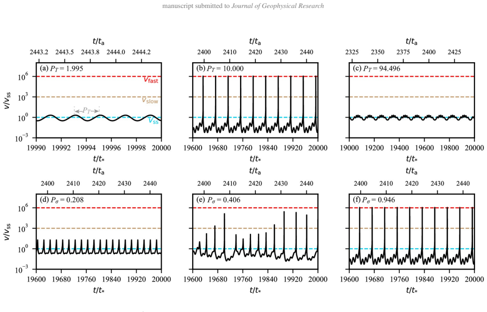
The central claim is that a stable-sliding velocity-weakening fault can be driven into episodic slip by periodic tidal-like stress perturbations, and that the response is governed by two dimensionless numbers: the normalized perturbation period P_T = T V_ss/d_c and the normalized Coulomb amplitude P_sigma = |Δτ − f*_ss Δσ|/(aσ0). Numerical simulations map a triggering window roughly P_sigma ≳ 0.2 and 2 ≲ P_T ≲ 70; inside that window slip velocity amplifies, radiation efficiency rises, and events phase-lock to the tide, while outside it the fault merely creeps. The paper also shows that increasing P_T shifts event timing from the tidal stress peak toward the peak stress rate, and increasing P
What carries the argument
The carrying mechanism is a resonance between the periodic forcing and the fault's intrinsic state-evolution timescale, exposed by a nondimensional reduction of the spring-block rate-and-state equations. Two dimensionless groups do the work: P_T (forcing period divided by d_c/V_ss) and P_sigma (tidal Coulomb stress divided by instantaneous frictional strength aσ0). A phase diagram in (P_sigma, P_T) serves as the paper's central object, delimiting where periodic perturbations trigger events and where they do not; the boxcar analysis explains the discrete 'comb-like' pattern of amplified periods as constructive interference between the two step responses that make up each loading half-cycle.
Load-bearing premise
The load-bearing premise is that the numerical triggering window (P_sigma ≳ 0.2, 2 ≲ P_T ≲ 70) computed for a single near-critical fault (a/b = 0.9, k/k_c = 1.1) applies to natural slow-earthquake patches, even though the paper's own sensitivity runs show stronger stiffness suppresses the amplification.
What would settle it
A direct lab test: on a velocity-weakening fault sliding stably at k/k_c ≈ 1.1, apply sinusoidal normal stress with P_T ≈ 10 and P_sigma ≈ 0.2–0.4; the model predicts slip events with V/V_ss above 10^3. If no such events appear across the predicted window, the central triggering claim fails. Observationally, a tidally sensitive patch with independently constrained aσ0 > 500 kPa would also break the inferred strength bound.
If this is right
- If the window is correct, neither tidal amplitude nor period alone determines triggering; both must fall inside the resonant window, which sharpens predictions for which faults respond to which tidal constituents.
- Observed phase preference (stress peak versus stress-rate peak) becomes a diagnostic of P_T, and therefore of the ratio d_c/V_ss.
- Combining the amplitude window with typical tidal stress amplitudes of 0.1–100 kPa directly implies aσ0 between roughly 0.5 and 500 kPa, in line with inferences from real tremor catalogs.
- The framework links fault patch size to loading period through the d_c–size scaling, explaining why shallow low-frequency earthquakes respond to semidiurnal tides while deeper ordinary earthquakes respond to seasonal loading.
Where Pith is reading between the lines
- Extension: the same nondimensional window should apply to other periodic loads (seasonal hydrology, slow-slip stress transients) with their own periods; this predicts a systematic shift in which patch sizes are triggered by which loading periods.
- Extension: the model's single-patch treatment suggests that multi-patch interactions, when added, would smear phase-locking and radiation efficiency; that could explain why fast earthquakes rarely show tidal correlations while LFE-like patches do.
- Testable extension: in a laboratory friction experiment with stiffness just above critical, sinusoidal normal-stress loading with P_T ≈ 10 and P_sigma ≈ 0.2 should produce episodic velocity events; the absence of such events at amplitudes inside the predicted window would falsify the resonance picture.
Editorial analysis
A structured set of objections, weighed in public.
Referee Report
Summary. The paper studies a spring-block model with rate-and-state friction (aging law) for a velocity-weakening fault whose stiffness exceeds the critical value, so that it is stably sliding in the absence of forcing. It shows that step, boxcar, and harmonic normal-stress perturbations can produce amplified slip-velocity responses and, for harmonic tidal-like forcing, can trigger slow and fast slip events on an otherwise stable fault. Nondimensionalization yields six parameters; for fixed intrinsic parameters (R_ab=0.9, κ=1.1, N=10^6, ϵ=10^-3), the triggering region in the (P_σ, P_T) plane is approximately P_σ ≳ 0.2, 2 ≲ P_T ≲ 70. Triggered events show period-dependent phase preferences (stress peak at small P_T, stress-rate peak at large P_T) and comb-like patterns in radiation efficiency and phase locking. The authors use the triggering window to infer aσ_0 ≈ 0.5–500 kPa and d_c ≈ 0.6–20 μm for plate-convergence loading rates, and discuss consistency with observed tidal correlations of LFEs and tremors.
Significance. If the central triggering result survives scrutiny, the paper's main contribution is a falsifiable, dimensionless framework connecting tidal correlations to frictional parameters (aσ_0, d_c), extending the resonance mechanism of Perfettini et al. (2001). The nondimensionalization is derived from the governing equations rather than fitted, and the authors provide their software and data in a Zenodo repository, which strengthens reproducibility. The study also makes concrete observable predictions: the P_T-dependent phase shift and the comb-like period selectivity are compared with published tidal-correlation observations. However, the quantitative triggering window and the resulting parameter constraints rest on numerical simulations with an incompletely documented filtering procedure and on a single point in intrinsic parameter space, which limits the strength of the constraints until these issues are resolved.
major comments (3)
- [Appendix D; Figs. 6a, 6b; §4.3.1] The phase diagram and the triggering window (P_σ ≳ 0.2, 2 ≲ P_T ≲ 70) are produced after discarding runs that show 'persistent stable oscillations' attributed to numerical error accumulation. The manuscript does not state which (P_σ, P_T) runs were discarded, how the artifact was distinguished from physical oscillations, or what 'minimum number of slip events' was required. Because §4.3.1 converts the phase-diagram boundaries directly into constraints on aσ_0 and d_c, an unquantified filter could change those boundaries and hence the central inferential step. Please document the filter, verify that no discarded case falls inside the claimed triggering window, and show that the window is insensitive to reasonable filtering choices.
- [§3.2, Fig. 6a; §4.3.1; Appendix F] The quantitative window is established from simulations at a single intrinsic parameter set (R_ab=0.9, κ=1.1, N=10^6, ϵ=10^-3) with a single event definition (V/V_ss > 10^3). Appendix F shows that V_max/V_ss increases with N, is strongly suppressed for κ=10, and increases as R_ab→1. Thus the phase-diagram boundaries—and therefore the inferred aσ_0 and d_c ranges—are likely to shift for natural patches with different κ, N, or R_ab. The paper needs either a systematic mapping of the triggering boundaries in (κ, N, R_ab) space or a clearly stated boundary on the applicability of the inferred parameter constraints. If the 'approximately' window is only meant for this specific parameter set, the constraints in §4.3.1 should be reworded accordingly.
- [§3.2, event definition; §4.3.2] The event classification threshold V/V_ss > 10^3 is chosen to define an event, and the quantitative boundaries P_σ ≳ 0.2 and 2 ≲ P_T ≲ 70 depend on this threshold. The manuscript acknowledges the classification is model-based, but it does not test how the window changes for alternative thresholds (e.g., 10^2 or 10^4). A short sensitivity analysis would make the central window claim more robust and clarify how the inferred parameter constraints depend on the event definition.
minor comments (6)
- [Eq. (11)] The second nondimensional period P_T2 = T/t_a is introduced but not used in the analysis; consider removing it or explaining its role, to avoid implying that it controls the results.
- [Appendix F, Fig. F1 caption] 'tomb-like structures' should be 'comb-like structures' (matching the main text).
- [§2.2.2] Typo: 'asymmetic' should be 'asymmetric'.
- [§3.3] Grammar: 'the events as slip events satisfying V/V_ss > 10^3, no distinguish slow and fast' is unclear; rephrase for clarity.
- [§4.3.1] 'A lot of numerous studies' is redundant; suggest 'Numerous studies'.
- [§4.2] Typo: 'that it is more easy to become instablity' should be 'that it is easier to become unstable'.
Circularity Check
No material circularity: P_σ and P_T are derived from the governing equations, the triggering window is a simulation output, and the aσ0/d_c constraints are a logical inversion; only minor non-load-bearing self-citations and a numerical-filter caveat prevent a clean 0.
full rationale
The paper's derivation chain is self-contained. Appendix B nondimensionalizes the quasi-dynamic momentum balance (Eq. B1) and the RSF law (Eqs. B2-B3) to obtain P_T = T V_ss/d_c and P_σ = |Δτ−f*_ss Δσ|/(aσ0) algebraically (Eq. B8); these parameters are not fitted and no observed tidal-correlation data enter their construction. The phase diagram and the window Pσ≳0.2, 2≲P_T≲70 (Fig. 6a, Sec. 3.2) are numerical outputs from the spring-block model at the stated parameter set (Table 2), not definitions. Section 4.3.1 then inverts this window with an assumed tidal-stress range (0.1–100 kPa) and representative slip rates to bound aσ0 (0.5–500 kPa) and d_c (0.6–20 μm); this is model-to-observation inference, not circular. The self-citations (Zhou et al. 2026 for data/code; Kheirdast et al. 2025 for the continuum radiated-energy expression) are not load-bearing: Appendix C derives the event energy budget from Kostrov's definition and the governing equation, and the triggering prediction does not depend on those citations. The unquantified numerical-error filter in Appendix D (late-time oscillations 'attributed to numerical error accumulation' and controlled by a minimum event count) is a robustness caveat, not a circular reduction; likewise the sensitivity of the window to κ and N shown in Appendix F is a parameter-dependence caveat. Overall, the central nondimensional parameters emerge from the equations rather than being imported from the paper's own prior claims.
Axiom & Free-Parameter Ledger
free parameters (2)
- Event classification thresholds =
V/V_ss = 10^3 (slow), 10^6 (fast)
- Representative tidal amplitude and period for constraint mapping =
Δσ = 1 kPa, T = 12 h
axioms (5)
- domain assumption Rate-and-state friction with aging law (Dieterich 1979) governs fault strength
- domain assumption Quasi-dynamic spring-block point model with radiation damping approximates a fault patch
- domain assumption Tidal loading is represented as a sinusoidal normal stress perturbation with τ_p=0 in simulations
- ad hoc to paper Events are defined by normalized velocity thresholds rather than by observational event criteria
- domain assumption The background slip rate V_ss and tidal period T are separable timescales (steady loading during tidal cycle)
Cite this review
Pith. "Pith review of Theoretical constraints on tidal triggering of slow earthquakes." pith.science (2026). https://pith.science/paper/X27FYM5W
@misc{pith2026260206703,
  author       = {Pith},
  title        = {Pith review of: Theoretical constraints on tidal triggering of slow earthquakes},
  year         = {2026},
  howpublished = {\url{https://pith.science/paper/X27FYM5W}},
  note         = {Machine review of arXiv:2602.06703}
}
read the original abstract
Tidal stress is a globally acting perturbation driven primarily by the gravitational forces of the Moon and the Sun. Understanding how tidal stresses can trigger seismic events is essential for constraining tectonic environments that are sensitive to small stress perturbations. Here, employing a spring-block model with rate-and-state friction, we investigate tidal triggering on velocity-weakening stable sliding faults with stiffness slightly exceeding the critical stiffness. We first apply a step and a boxcar with finite duration normal stress perturbation to demonstrate a resonance-like amplification of slip velocity for specific boxcar durations. Next, we perform nondimensional analyses and numerical simulations with harmonic perturbations to identify the key parameters controlling tidal triggering and their admissible ranges. Triggered slip events are further characterized using physically observable quantities, including radiation efficiency and tidal phase. Our results show that even small stress perturbations can trigger periodic as well as temporally complex slip events on stable sliding faults. The triggering behavior is primarily controlled by the normalized perturbation period and the normalized perturbation amplitude. An increase in the normalized period shifts event timing from the peak of tidal stress toward the peak of stress rate, whereas increasing the normalized amplitude promotes a transition from slow to fast events. This framework helps explain the period-dependent sensitivity and the observed phase preference between tidal stress and maximum slip velocity. Comparison between observed and model-predicted tidal correlation patterns may therefore help constrain the instantaneous frictional strength of the interface, as well as the characteristic slip distance for frictional weakening.
Figures




Reference graph
Works this paper leans on
-
[1]
Can observations of earthquake scaling constrain slip weakening?
Abercrombie, R. E. & J. R. Rice (2005). “Can observations of earthquake scaling constrain slip weakening?” In:Geo- physical Journal International162.2, pp. 406–424.DOI:10.1111/j.1365-246X.2005.02579.x. Ader, T. J., J.-P. Ampuero & J.-P. Avouac (2012). “The role of velocity-neutral creep on the modulation of tectonic tremor activity by periodic loading”. I...
Pith/arXiv arXiv 2005
-
[2]
Above equation can be compared toKostrov (1974, Eq
This formulation follows directly from quasi-dynamic governing equation and no assumption are made to obtain the above equation. Above equation can be compared toKostrov (1974, Eq. 2.24).The main feature of this equation is that all the terms can be calculated using incremental quantities. AssumingA[m 2]is the rupture area of the event, the last term in E...
1974
-
[5]
Seismicity modulation in a 3-D rate-and-state interacting fault population model
Experimental results and constitutive equations”. In:J. Geophys. Res.84.B5, pp. 2161–2168.DOI:10.1029/JB084iB05p02161. Dublanchet, P. (2022). “Seismicity modulation in a 3-D rate-and-state interacting fault population model”. In:Geophysical Journal International229.3, pp. 1804–1823.DOI:10.1093/gji/ggac023. Erickson, B., B. Birnir & D. Lavall ´ee (2008). “...
-
[7]
Tidal modulation and tectonic implications of tremors in Taiwan
Chen, K. H., H.-J. Tai, S. Ide, T. B. Byrne & C. W. Johnson (2018). “Tidal modulation and tectonic implications of tremors in Taiwan”. In:Journal of Geophysical Research: Solid Earth123.7, pp. 5945–5964.DOI:10.1029/2018JB0156
-
[9]
The integration interval was set tot∈[0,20000t ∗], where t∗ =d c/Vss
Error control was applied only to the physically relevant state variables(τ, V, σ), excluding auxiliary integral variables. The integration interval was set tot∈[0,20000t ∗], where t∗ =d c/Vss. In a few simulations, we observe that long sequences of slip events are followed by a transition to persistent stable oscillations. Upon verification, these late-t...
2026
-
[11]
Appendix D Numerical Methods We solved the governing equations using theDifferentialEquations.jlpackage in Julia (v1.11.0, DifferentialE- quations.jl v7.15.0)
We explicitly verify the validity of the incremental energy balance for each events defined by velocity thresholds and examine the external work term∆W ext and find that its contribution is negligible in our simulations. Appendix D Numerical Methods We solved the governing equations using theDifferentialEquations.jlpackage in Julia (v1.11.0, DifferentialE...
1990
-
[13]
As shown in Fig
almost stable sliding regime. As shown in Fig. F1a,V max/Vss increases systematically withN. Although the scaling is not strictly linear, the overall trend suggests a strong positive dependence ofV max/Vss onN. The effect of system stiff- ness is examined by varyingκ= 1.1,2.5, and10. As illustrated in Fig. F1b, larger values ofκsystematically suppress the...
2026
-
[63]
Earth tides can trigger shallow thrust fault earthquakes
Cochran, E. S., J. E. Vidale & S. Tanaka (2004). “Earth tides can trigger shallow thrust fault earthquakes”. In:Science 306.5699, pp. 1164–1166.DOI:10.1126/science.1103961. Das, S. (1976). “A Numerical Study Of Rupture Propagation And Earthquake Source Mechanism”. PhD thesis. Mas- sachusetts Institute of Technology. DeMets, C., R. G. Gordon & D. F. Argus ...
Pith/arXiv arXiv 2004
-
[120]
Washington, D. C.: American Geophysical Union, pp. 147–163.ISBN: 978-0-87590-978-3.DOI:10.1029/GM120p0147. Kheirdast, N, H. S. Bhat, M Almakari, A Gupta, C Villafuerte, M. Y . Thomas & P Dubernet (2025). “Energy budget of spectrum of slip dynamics emerging from simplified model of fault and damage zone architecture”. In:to be subm. DOI:10.48550/arXiv.2509...
-
[754]
22Feb. 9, 2026 at 01:51 manuscript submitted toJournal of Geophysical Research Sahoo, S., B. Senapati, D. Panda, S. Jin & B. Kundu (2024). “Tidal triggering of seismic swarm associated with hy- drothermal circulation at Blanco ridge transform fault zone, Northeast Pacific”. In:Physics of the Earth and Planetary Interiors356, p. 107259.DOI:10.1016/j.pepi.2...
arXiv 2026
-
[848]
Connecting slow earthquakes to huge earthquakes
Obara, K. & A. Kato (2016). “Connecting slow earthquakes to huge earthquakes”. In:Science353.6296, pp. 253–257. DOI:10.1126/science.aaf1512. Ohnaka, M. (2003). “A Constitutive Scaling Law and a Unified Comprehension for Frictional Slip Failure, Shear Fracture of Intact Rock, and Earthquake Rupture”. In:Journal of Geophysical Research: Solid Earth108.B2, 2...
-
[9587]
Fracture Mechanics of Rate-and-State Faults and Fluid Injection Induced Slip
Garagash, D. I. (2021). “Fracture Mechanics of Rate-and-State Faults and Fluid Injection Induced Slip”. In:Philosophical Transactions of the Royal Society A: Mathematical, Physical and Engineering Sciences379.2196, p. 20200129.DOI: 10.1098/rsta.2020.0129. Garagash, D. I. & L. N. Germanovich (2012). “Nucleation and Arrest of Dynamic Slip on a Pressurized F...
arXiv 2021
discussion (0)
Sign in with ORCID, Apple, or X to comment. Anyone can read and Pith papers without signing in.