REVIEW 5 major objections 6 minor 115 references
Cosmo-PINN: A Physics-Informed Neural Network for Cosmological Reconstruction
T0 review · 5 major / 6 minor · reviewed 2026-08-02 · deepseek-v4-flash
Pith's one-line read A physics-informed neural network, trained with the Friedmann equations as hard constraints, reconstructs a dark energy equation of state that crosses w=−1 between z=0.27 and 0.42.
desk verdict Useful PINN reconstruction of w_DE(z) with an honest limitations section, but the phantom-crossing claim is not yet robust because the Ω_m0 prior is unspecified and the uncertainty quantification is non-standard. read the letter →
The pith
A machine-rendered reading of the paper's core claim, the machinery that carries it, and where it could break.
The reading
What carries the argument
The central object is the Cosmo-PINN loss function, which adds two PDE residuals to the data likelihood: R1 enforces the conservation equation relating Ω_m and w_DE, and R2 enforces the second Friedmann equation for H(z). The unknown functions are represented as Chebyshev polynomial expansions (H(x)=H0 exp[x N_H(x)] and w_DE(x)=Σ c_n T_n(2x−1)), with automatic differentiation for derivatives; the cosmological parameters H0, Ωm0, and r_drag are learned with soft Gaussian priors anchored at Planck 2018 values. Adaptive loss weighting balances the data and physics terms, and posterior uncertainties are produced by Hamiltonian Monte Carlo sampling of the Chebyshev coefficients and final-layer we
What would settle it
Train Cosmo-PINN on mock datasets generated from a flat ΛCDM expansion (w=−1) with the same noise realizations as the real observations. If the recovered w_DE(z) still crosses −1 within the 95% credible intervals, the phantom crossing is generated by the method or the priors rather than required by the data. As a cheaper check, rerun with the Ω_m0 prior center shifted by ±0.01: if the crossing redshift moves outside the quoted range, the result is prior-dominated.
Extended reading notes
Core claim
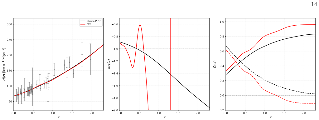
The central claim is that a physics-informed neural network can recover the dark-energy equation of state from background observations without assuming a parametric form, and that the recovered w_DE(z) crosses the phantom divide at z≈0.3–0.4 for all four data combinations considered. In the quintessence-bounded version, the network reconstructs a high-redshift Ω_DE that stays positive and pressureless, which the paper interprets as evidence for a unified dark sector described by an exponential (or, for Union3, hyperbolic) scalar potential. The author also claims that omitting the physics loss leads to a ghost-like Ω_DE<0 and oscillating w_DE, demonstrating that the field-equation constraints
Load-bearing premise
The reconstruction collapses if the soft Planck-centered prior on Ω_m0 is inappropriate: because w_DE(z) and Ω_m0 are degenerate, a shifted or overly tight prior would move the phantom-crossing redshift and the high-z dark-energy plateaus, and the paper does not quantify this sensitivity.
Editorial extensions
If this is right
- If the reconstruction is right, ΛCDM is disfavored by the background data, and the dark energy sector is dynamical rather than constant.
- The quintessence-bounded result implies a scalar field could act as both dark matter and dark energy, making unified dark-sector models empirically accessible.
- Omitting the physics residuals from the loss produces unphysical negative dark-energy densities, so future model-agnostic reconstructions should enforce the field equations.
- The same network design transfers to scalar-field potentials, modified-gravity free functions, and interacting dark sectors whenever the equations admit a residual form.
Reading between the lines
- A decisive stress test is to run the same pipeline on mock catalogs generated from a known ΛCDM expansion; if it still returns a phantom crossing, the crossing is an artifact of the priors or loss weighting.
- Because the Planck-centered Ω_m0 prior has unspecified width and is degenerate with w_DE(z), shifting that prior by a small amount should move the crossing redshift; quantifying that sensitivity would show whether the central result is data-driven or prior-driven.
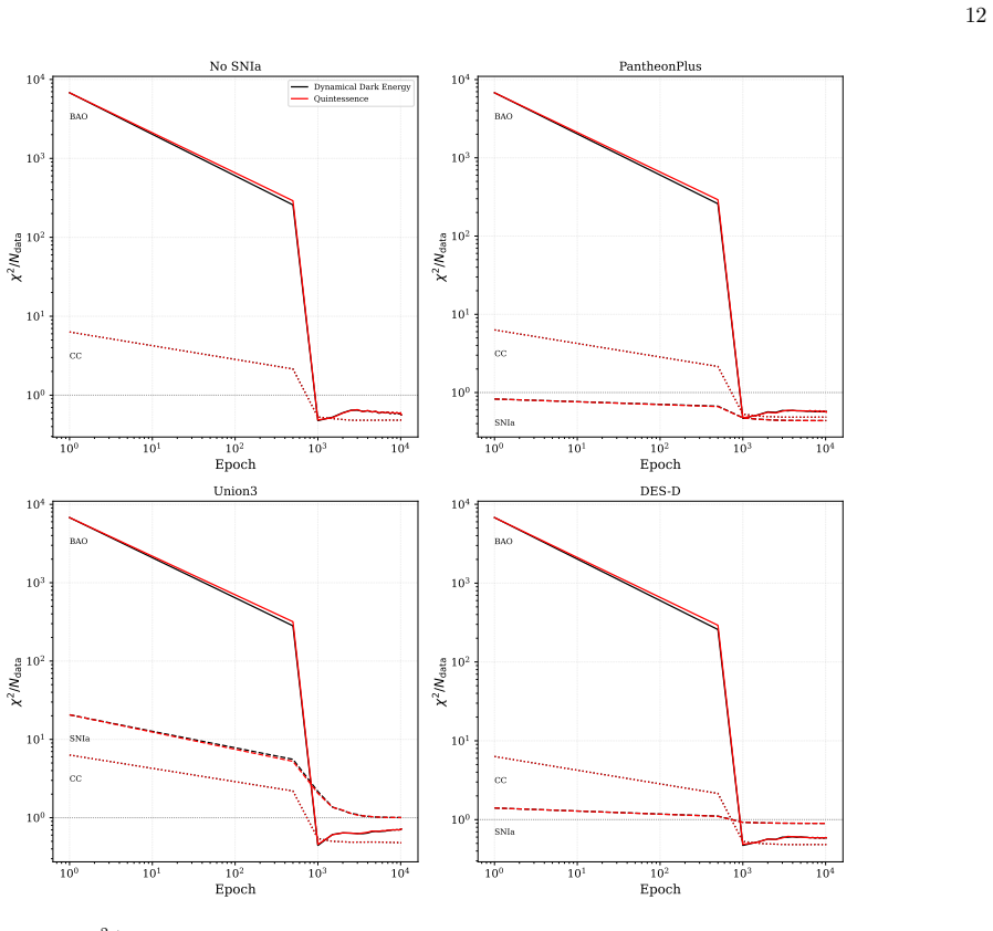
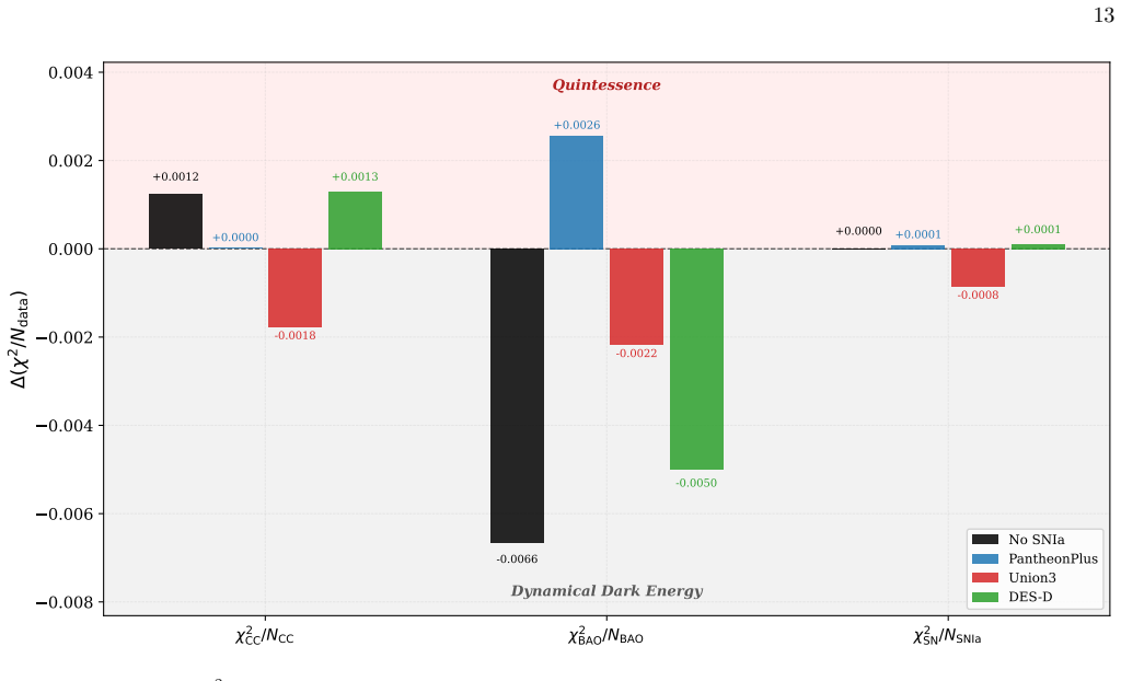
- The reduced-χ²-per-dataset weighting with log caps is an optimization criterion, not a likelihood; a formal model comparison between ΛCDM and the reconstructed w_DE is needed before the phantom crossing can be claimed as a statistical preference.
Editorial analysis
A structured set of objections, weighed in public.
Referee Report
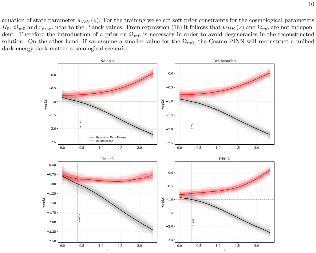
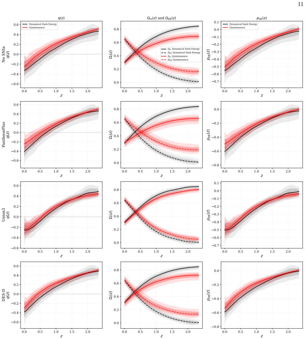
Summary. The manuscript introduces Cosmo-PINN, a physics-informed neural network that reconstructs the dark energy equation-of-state parameter w_DE(z) from DESI DR2 BAO data, cosmic chronometers, and three SNIa compilations. The network represents H(z) through a Chebyshev-log expansion and w_DE(z) as a Chebyshev series; the Friedmann/continuity equations are imposed as additional terms in a weighted loss. H0, Ω_m0, and r_drag are trained parameters with soft priors near Planck 2018 values. The central reported result is that, in the unbounded case, w_DE(z) decreases monotonically and crosses the phantom divide at z ≈ 0.27–0.42, claimed to agree with the CPL model. In the quintessence-bounded case, Ω_DE(z) remains nonzero at high redshift, suggesting a unified dark sector. A comparison with a physics-free neural network shows that imposing the Friedmann residuals prevents the unphysical negative Ω_DE found in the unconstrained fit.
Significance. If the phantom-crossing result is robust, the paper would provide a meaningful, mostly model-independent, physics-informed reconstruction from late-time data and would strengthen the case for dynamical dark energy over ΛCDM. The manuscript has genuine strengths: the Friedmann residuals R1 and R2 in Eqs. (19)–(20) are correctly derived (including signs), the stability tests across initial conditions and Chebyshev degrees are useful, and the authors are appropriately explicit in §III.A that the loss is a reconstruction criterion rather than a strict likelihood and that the χ² differences in Fig. 9 are optimization diagnostics. The comparison with an unconstrained NN in §V is a good sanity check. However, the central claim is currently conditional on an unspecified degeneracy-breaking prior on Ω_m0, and the reported credible intervals are not derived from an explicitly defined posterior. The paper also overstates the 'hard constraint' nature of the penalty terms. These issues are fixable, but they are load-bearing for the headline result.
major comments (5)
- [§IV, Eq. (23)] The reconstruction is degenerate in (w_DE, Ω_m0), as the paper itself states in §IV. The degeneracy is broken by the L_IC term, but the widths σ_H0, σ_Ωm0, σ_rdrag and the weights λ_H0, λ_Ωm0, λ_rdrag in Eq. (23) are never reported. The robustness tests in §III.C use a 'medium' prior, while the production reconstruction uses an unspecified 'soft' prior. The phantom-crossing redshift z=0.27–0.42 in Fig. 6 and the high-z Ω_DE plateau in the quintessence case are therefore conditional on unpublished hyperparameters. A factor-of-two change in σ_Ωm0 could plausibly move or erase the crossing. Please publish the exact prior hyperparameters and run a sensitivity scan, including the Ω_m0 prior centered at different values and σ_Ωm0 varied by a factor of at least 3, reporting whether the crossing and plateau persist.
- [§III.D, Eq. (31)] The HMC-based 'posterior uncertainties' and the 68/95% bands in Figs. 6–7 are not derived from an explicitly defined probabilistic model. L_PINN in Eq. (31) is a weighted sum of data χ² terms, PDE residuals, initial-condition penalties, smoothness penalties, and bounds; it is not a log-likelihood. The text says priors are placed on three cosmological parameters and that the log-likelihood is the data contribution, but it does not state whether the PDE/bounds/smoothness terms enter the HMC likelihood, with what effective scales, or how the adaptive weights are treated. Without this, the reported credible intervals cannot be interpreted as Bayesian posterior intervals. Either specify a full probabilistic model with fixed likelihood scales, or relabel the bands as optimization-sensitivity envelopes and avoid Bayesian language.
- [§III.B and Abstract] The physical laws are repeatedly called 'hard constraints' in the abstract and in §III, but they are implemented as soft penalty terms in L_PDE and L_bounds, with weights that are adaptively changed during the first 5000 epochs and then frozen. The PDE residual is also evaluated only at N_c collocation points, so the equations are not guaranteed to vanish at every point. The comparison in §V shows improved physical behavior but not exact satisfaction. Please report the final PDE residuals and either replace the penalty implementation with a strictly enforced projection or reword the 'hard constraint' / 'satisfy the physical laws at every point' claim. This is a central selling point of the method and is currently overstated.
- [§III.2] The baryon density expression Ω_b(z)=ω_b (1+z)^3/H(z)^2 is dimensionally inconsistent as written. Since H(z) is the physical Hubble parameter used in Eqs. (24)–(25), H(z)^2 has units of (km/s/Mpc)^2, so the right-hand side does not have the dimensionless form required for Ω_b. The intended expression is presumably Ω_b(z)=ω_b (1+z)^3/(H(z)/H0)^2, with ω_b defined appropriately (Ω_b0 or Ω_b0 h^2 depending on the H normalization). Because Ω_b enters the closure constraint (8) and therefore Ω_DE, this affects the reconstructed w_DE(z). Please correct the formula and confirm that the implementation uses the normalized H in this term.
- [§IV, Fig. 6] The claimed 'agreement with the CPL model' is referenced to [51], a paper by the same author using overlapping DESI DR2 data. This is not an independent validation. Please either perform and report an independent CPL fit to the same datasets within this paper, or explicitly characterize the agreement as consistency with a previous model-dependent reconstruction by the same group rather than independent confirmation. This distinction matters for the strength of the central claim.
minor comments (6)
- [Abstract / §III.A] The terminology should be unified: 'hard constraints' is used in the abstract and §III, while §III.A explicitly says the loss is a reconstruction criterion and calls the parameter terms 'soft priors.' These statements are in tension and should be reconciled.
- [§III.C / §IV] The distinction between 'medium' and 'soft' priors is never quantified. A table listing the actual values of σ_H0, σ_Ωm0, σ_rdrag and λ_H0, λ_Ωm0, λ_rdrag for each training setup would resolve much of the ambiguity.
- [§III.B, Eq. (31)] L_SP and L_bounds are only described verbally; their exact functional forms and weights are not given. Please specify these terms so the total loss is reproducible.
- [§III.D] The sentence about sampling 'the weights of the final network layer that directly parametrize H(z) and w_DE(z)' is confusing, because H and w_DE are parametrized by Chebyshev coefficients, not by network output weights. Please clarify which variables are sampled.
- [§II, datasets] The PantheonPlus and Union3 compilations share 1363 SNIa events; this non-independence should be stated explicitly when the three SNIa combinations are compared in §IV.
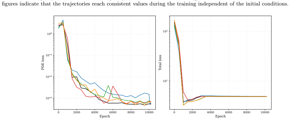
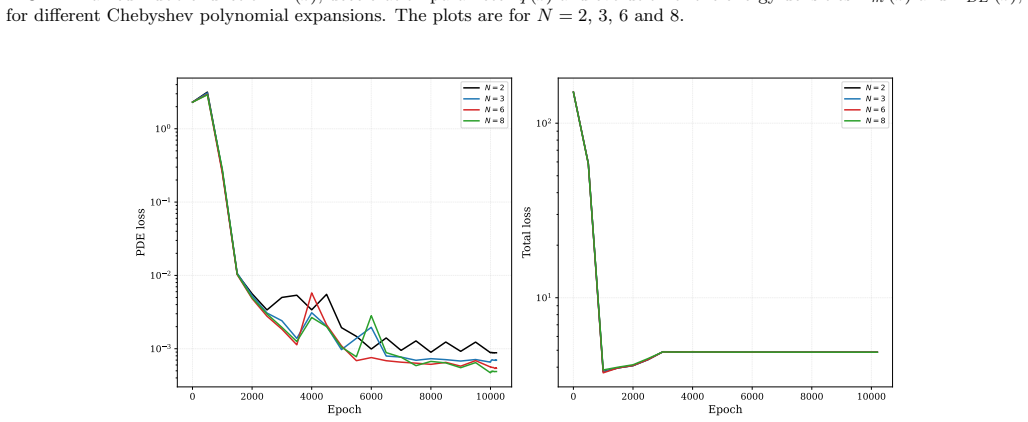
- [References] Minor typographical issues: ref. [42] lists 'Chevaller' instead of 'Chevallier'; ref. [8] has 'Atropharticle' instead of 'Astroparticle'; the caption of Fig. 3 refers to 'PDE loss parameter' where 'PDE loss' seems intended.
Circularity Check
No definitional circularity: the reconstructed w_DE(z) is a free Chebyshev function fitted under Friedmann residuals; the only rubric-level issue is a non-independent same-author citation used as the CPL 'agreement' benchmark.
full rationale
The central derivation is self-contained rather than circular. w_DE(z) is introduced as a free Chebyshev expansion (Eq. 21) and is determined, together with H(z) and Omega_m(z), by minimizing data residuals subject to the Friedmann-equation residuals R1 and R2 (Eqs. 19-20). The phantom-crossing redshift is thus a fitted output of an optimization over external data, not an input or a parameter renamed as a prediction. Section IV explicitly recognizes the w_DE-Omega_m0 degeneracy and breaks it with soft Planck priors; the widths are not reported, which is a robustness/sensitivity gap, but the prior is an ordinary modeling input rather than a definitional construction of the result. Section III.A.4 states the loss 'should be interpreted as a reconstruction criterion and not right strict likelihood combination,' while Section III.D later uses HMC to produce posterior intervals; this is an internal tension in the uncertainty quantification, not a circular reduction. The one self-citation issue is that the abstract and Section IV claim agreement with the CPL model and cite ref. [51], a prior paper by the same author on overlapping DESI DR2 data. That weakens the external validation, but the reconstruction does not depend on [51] to produce the crossing, so the self-citation is minor and not load-bearing. No equation reduces to an input by construction, so the circularity score is low.
Assumptions & free parameters
free parameters (7)
- H0 =
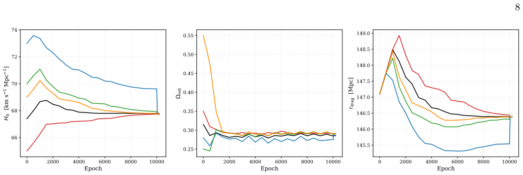
≈70 km/s/Mpc (from Fig. 2; soft-prior to Planck 2018)
- Ω_m0 =
≈0.28–0.35 (Fig. 2 varies across runs; prior to Planck)
- r_drag =
≈145.5–149 Mpc
- Chebyshev coefficients =
N=5 → 6 coefficients for w_DE and for H, plus coefficients for Ω_m function
- Loss weights and log-cap γ =
λs adapted via GradNorm first 5000 epochs; γ² > 1
- Prior widths σ_H0, σ_Ωm0, σ_rdrag =
not specified ('medium')
- Smoothness penalty weights and bounds =
not specified
assumptions (8)
- domain assumption FLRW flat geometry with GR field equations (Eqs. 1-3)
- domain assumption Cosmic fluid is a sum of non-interacting perfect fluids: radiation, baryons, CDM, and dark energy, each separately conserved (Eqs. 10-13)
- domain assumption Dark energy is a barotropic fluid with p_DE = w_DE(z) ρ_DE
- domain assumption Radiation energy density is negligible at z ≤ 2.33 and is omitted from the analysis
- domain assumption Planck 2018 values anchor the soft priors for H0, Ω_m0 and r_drag (Eq. 23)
- ad hoc to paper The loss is a weighted reconstruction criterion, not a strict likelihood
- domain assumption Quintessence bound w_DE ∈ [−1, 1] when imposed
- ad hoc to paper Chebyshev expansion and smoothness penalties provide sufficient regularization
Cite this review
Pith. "Pith review of Cosmo-PINN: A Physics-Informed Neural Network for Cosmological Reconstruction." pith.science (2026). https://pith.science/paper/X5KYKFHM
@misc{pith2026260530139,
  author       = {Pith},
  title        = {Pith review of: Cosmo-PINN: A Physics-Informed Neural Network for Cosmological Reconstruction},
  year         = {2026},
  howpublished = {\url{https://pith.science/paper/X5KYKFHM}},
  note         = {Machine review of arXiv:2605.30139}
}
abstract
We introduce Cosmo-PINN, a Physics-Informed Neural Network for reconstruction of the cosmological theory. In this work we demonstrate the application of the Cosmo-PINN in the reconstruction of the dark energy equation of state parameter $w_{DE}\left( z\right) $ directly from late-time cosmological observations. This framework overcomes the main limitation shared by Gaussian Process and Artificial Neural Network reconstruction approaches, where the recovered solution is driven by the data and it is not necessarily true that it is physically consistent, by embedding the cosmological constraints directly into the loss function as hard constraints, ensuring that the reconstructed quantities satisfy the physical laws at every point during the training. For the training of the network, we employed background data, and specifically the Baryon Acoustic Oscillation from DESI DR2, the Cosmic Chronometers and three different Supernova compilations, while we simultaneously introduce the cosmological parameters $H_{0},~\Omega _{m0}$ and $r_{\mathrm{drag}}$ as trained parameters. The reconstruction shows that the trained $w_{DE}\left( z\right) $ crosses the phantom divide within the redshift range $z=0.27-0.42$ in agreement with the value obtained by the Chevallier-Polarski-Linder model. In the quintessence scenario, for large redshifts the dark energy $\Omega _{DE}\left( z\right) $ provides a pressureless nonzero contribution to the cosmological fluid suggesting a unified scenario. Finally, we demonstrate the significance of imposing the physical constraints within the loss function by comparing the Cosmo-PINN reconstruction against a purely data-driven neural network with the same architecture.
Figures
Figures from the paper (7 more)
Reference graph
Works this paper leans on
-
[51]
Linder, Phys
E.V. Linder, Phys. Rev. Lett. 90, 091301 (2003)
2003
-
[1]
Physical law The full set of physical quantities is trained under the requirement of physical consistency. In order to guarantee the trained solution possesses the initial condition for the Hubble function we assume the expression H(x) =H 0 exp [x NH (x)], in which NH (x) = NX n=1 c(H) n Tn(2x−1),(17) is a Chebyshev polynomial expansion, and coefficientsc...
-
[2]
Initial conditions As far as the baryons are concerned, we express them as Ω b(z) = ωb (1+z)3 H(z) 2 , whereω b is the value obtained by the Planck 2018 collaboration. On the other hand, regarding the free parametersH 0,Ω m0 andr drag we introduce them into the total loss via the expression LIC = λH0 2 H PINN 0 −H P lanck 0 σH0 2 + λΩm0 2 ΩPINN m0 −Ω P la...
2018
-
[3]
Last but not least, in order to avoid unphysical oscillations related to overfitting, we introduce weak smoothness penaltiesL SP
Smoothness penalties and physical boundaries We introduce aL bounds component in the loss function, in order to impose strong boundary conditions on the trained functions such that the obtained solution satisfies Ω m ∈[0,1], or in the case of quintessence thew DE is within the rangew DE ∈[−1,1]. Last but not least, in order to avoid unphysical oscillation...
-
[4]
We consider the 31 model independent direct measurements of the Hubble parameter within the redshift range 0.09≤z≤1.965 [90]
Cosmic Chronometers Finally, we employ the cosmic chronometers, which are old galaxies, passively evolving with synchronous stellar populations and similar cosmic evolution [89]. We consider the 31 model independent direct measurements of the Hubble parameter within the redshift range 0.09≤z≤1.965 [90]. The Hubble function is trained by the PINN and theχ ...
-
[5]
Baryon Acoustic Oscillations We consider the recent BAO DESI DR2 catalogue [91, 92]. This dataset consists of 13 measurements from DESI DR2 at seven redshifts with the rangez∈[0.295,2.33],of the Hubble distance ratio the comoving angular distance ratio and the volume-averaged distance ratio, each normalized by the sound horizon at the baryon drag epochr d...
-
[6]
The catalogues provide measure- ments of the distance modulusµ obs i as a function of redshiftz i
Type Ia Supernovae We make use of three different (SNIa) compilations, the PantheonPlus (PP) catalogue without the SH0ES Cepheid calibration [93], the Union3.0 (U3) [94] and the recent DES-Dovekie (DESD) [95]. The catalogues provide measure- ments of the distance modulusµ obs i as a function of redshiftz i. The U3 and PP catalogues provide events within t...
-
[7]
For 1 NData χ2 Data << γ2, theL DATA ≃ 1 NData χ2 Data
Data Loss function The component of the loss function related to the training given by the cosmological data is defined as LDATA =λ CC LCC +λ BAO LBAO +λ SN LSN,(28) whereλare the data weights, the loss function related to the CC is defined as LCC = 1 NCC χ2 CC,(29) 7 and for the loss functionL BAO,L SN we introduce a logarithmic cap, that is, LBAO =γ 2 l...
2000
Show all 115 references
-
[8]
First, we perform training runs with different sets of initial conditions to verify whether the PINN converges to a consistent solution
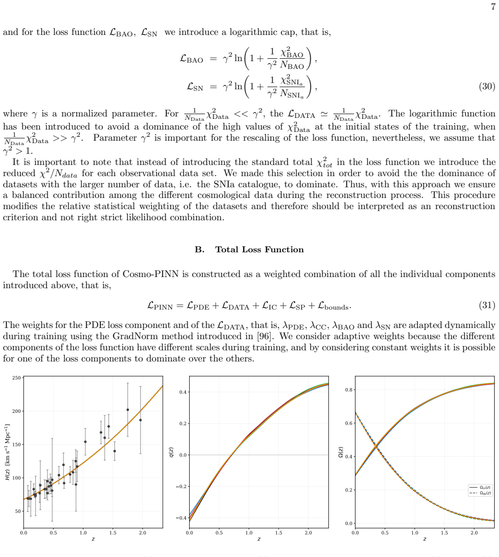
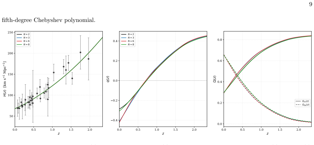
Stability and Robustness Tests Before we proceed with the reconstruction of the dark energy equation of state parameterw DE (z) we present two tests to assess the viability of the Cosmo-PINN. First, we perform training runs with different sets of initial conditions to verify w...
-
[9]
Riess et al., Astron
A.G. Riess et al., Astron. J. 116, 1009 (1998)
1998
-
[10]
Tegmark et al., Astrophys
M. Tegmark et al., Astrophys. J. 606, 702 (2004)
2004
-
[11]
Kowalski et al., Astrophys
M. Kowalski et al., Astrophys. J. 686, 749 (2008)
2008
-
[12]
Komatsu et al., Astrophys
E. Komatsu et al., Astrophys. J. Suppl. Ser. 180, 330 (2009)
2009
-
[13]
Suzuki et al., Astrophys
N. Suzuki et al., Astrophys. J. 746, 85 (2012)
2012
-
[15]
Gutierrez, Nucl
G. Gutierrez, Nucl. Part. Phys. Proceedings, 267, 332 (2015)
2015
-
[16]
Di Valentino et al., Atropharticle Physics 131, 102605 (2021)
E. Di Valentino et al., Atropharticle Physics 131, 102605 (2021)
2021
-
[17]
Weinberg, Rev
S. Weinberg, Rev. Mod. Phys. 61, 1 (1989)
1989
-
[18]
Padmanabhan, Phys
T. Padmanabhan, Phys. Rept. 380, 235 (2003)
2003
- [19]
-
[20]
Di Valentino et al
E. Di Valentino et al. [CosmoVerse Network], Phys. Dark Univ. 49, 101965 (2025)
2025
-
[21]
Gorini, A
V. Gorini, A. Kamenshchik and U. Moschella, Phys. Rev. D 67, 063509 (2003)
2003
-
[22]
Valiviita, E
J. Valiviita, E. Majerotto, and R. Maartens, JCAP 07, 020 (2008)
2008
-
[23]
B. Wang, E. Abdalla, F. Atrio-Barandela, and D. Pavon, Rept. Prog. Phys. 79, 096901 (2016)
2016
-
[24]
Paliathanasis, Phys
A. Paliathanasis, Phys. Dark Univ. 52, 102306 (2026)
2026
-
[25]
Ratra and P.J.E
B. Ratra and P.J.E. Peebles, Phys. Rev. D 37, 3406 (1988)
1988
-
[26]
Peebles and B
P.J.E. Peebles and B. Ratra, Rev. Mod. Phys. 75, 559 (2003)
2003
-
[27]
Ludwick, Mod
K.J. Ludwick, Mod. Phys. Lett. A 32, 28 (2017)
2017
-
[28]
V´ azquez, D
J.A. V´ azquez, D. Tamayo, G. Garcia-Arroyo, I. G´ omez-Vargas, I. Quiros, A.A. Sen, Phys. Rev. D 109, 023511 (2024)
2024
-
[29]
Shajib and J.A
A.J. Shajib and J.A. Frieman, Phys. Rev. D 112, 063508 (2025)
2025
-
[30]
van de Bruck, G
C. van de Bruck, G. Poulot and E.M. Teixeira, JCAP 07, 019 (2023)
2023
-
[31]
Paliathanasis, T
A. Paliathanasis, T. Mengoni, G. Leon and O. Luongo, Constraints on Chiral-Quintom dark energy after DESI DR2 and impact on unifying dark energy with inflation, (2025) [arXiv:2512.00558]
2025
-
[32]
Deffayet, X
C. Deffayet, X. Gao, D.A. Steer and G. Zahariade, Phys. Rev. D 84, 064039 (2011)
2011
-
[33]
Faraoni, Cosmology in Scalar-Tensor Gravity, Springer Dordrecht (2004)
V. Faraoni, Cosmology in Scalar-Tensor Gravity, Springer Dordrecht (2004)
2004
-
[34]
Kase and S
R. Kase and S. Tsujikawa, Int. J. Mod. Phys. D 28, 1942005 (2019)
2019
-
[35]
Buchdahl, Mon
H.A. Buchdahl, Mon. Not. Roy. Astron. Soc. 150, 1 (1970)
1970
-
[36]
Ferraro and F
R. Ferraro and F. Fiorini, Phys. Rev. D 75, 084031 (2007)
2007
-
[37]
Heisenberg, Physics Rept
L. Heisenberg, Physics Rept. 1066, 1 (2024)
2024
-
[38]
Clifton, P.G
T. Clifton, P.G. Ferreira, A. Padilla and C. Skordis, Phys. Rept. 513, 1 (2012)
2012
-
[39]
Nojiri, S.D
S. Nojiri, S.D. Odintsov and V.K. Oikonomou, Phys.Rept. 692, 1 (2017)
2017
-
[40]
Joyce, L
A. Joyce, L. Lombriser and F. Schmidt, Annu. Rev. Nucl. Part. Sci. 66, 122 (2016)
2016
-
[41]
Yoo and Y
J. Yoo and Y. Watanabe, Int. J. Mod. Phys. D 21, 1230002 (2012)
2012
-
[42]
Nojiri, S.D
S. Nojiri, S.D. Odintsov and M. Sasaki, Phys. Rev. D 71, 123509 (2005)
2005
-
[43]
Saridakis, Phys
E.N. Saridakis, Phys. Rev. D 102, 123525 (2020)
2020
-
[44]
Basilakos, A
S. Basilakos, A. Lymperis, M. Petronikopoulou and E.N. Saridakis, Nucl. Phys. B 1015, 116904 (2025)
2025
-
[45]
Sahlu, A
S. Sahlu, A. de la Cruz-Dombriz and A. Abebe, MNRAS 539, 690 (2025)
2025
-
[46]
Paliathanasis, JHEAp 52, 100609 (2026)
A. Paliathanasis, JHEAp 52, 100609 (2026)
2026
-
[47]
Paliathanasis, Phys
A. Paliathanasis, Phys. Dark Univ. 52, 102337 (2026)
2026
-
[48]
Shafiello, V
A. Shafiello, V. Sahni and A. Starobinsky, Annalen Phys. 19, 316 (2010)
2010
-
[49]
Giare, M
W. Giare, M. Najadi, S. Pan, E. Di Valentino and J.T. Firouzjaee, JCAP 10, 035 (2024)
2024
-
[50]
Chevaller and D
M. Chevaller and D. Polarski, Int. J. Mod. Phys. D 10, 213 (2001)
2001
-
[52]
Rezaei, M
M. Rezaei, M. Malekjani, S. Basilakos, A. Mehrabi, and D. F. Mota, Astrophys. J. 843, 65 (2017)
2017
-
[53]
L. Xing, J. Chen, Y. Gui, E. Schlegel and J. Lu, Mod. Phys. Lett. A 26, 885 (2011) 16
2011
-
[54]
Barboza Jr
E.M. Barboza Jr. and J.S. Alcaniz, Phys. Lett. B 666, 415 (2008)
2008
-
[55]
Dimakis, A
N. Dimakis, A. Karagiorgos, A. Zampeli, A. Paliathanasis, T. Christodoulakis and Petros A. Terzis, Phys. Rev. D 93, 123518 (2016)
2016
-
[56]
Linder, Astropart
E.V. Linder, Astropart. Phys. 25, 167 (2006)
2006
-
[57]
Tripathi, A
A. Tripathi, A. Sangwan and H.K. Jassal, JCAP 06, 012 (2017)
2017
-
[58]
Escamilla, S
L.A. Escamilla, S. Pan, E. Di Valentino, A. Paliathanasis and J.A. Vazquez, Phys. Rev. D 111, 2 (2025)
2025
-
[59]
Paliathanasis, Phys
A. Paliathanasis, Phys. Dark Univ. 48, 101956 (2025)
2025
-
[61]
Shafieloo, A.G
A. Shafieloo, A.G. Kim and E.V Linder, Phys. Rev. 85, 123530 (2012)
2012
-
[62]
Seikel, C
M. Seikel, C. Clarkson and M. Smith, JCAP 06, 036 (2012)
2012
-
[63]
Yang, Z.-K
T. Yang, Z.-K. Guo and R.-G. Cai, Phys. Rev. D 91, 123533 (2015)
2015
-
[64]
Zhang and J.-Q
M.-J. Zhang and J.-Q. Xia, JCAP 12, 005 (2016)
2016
-
[65]
Jesus, R
J.F. Jesus, R. Valentim, A.A. Escobal and S.H. Pereira, JCAP 04, 053 (2020)
2020
-
[66]
Yennapureddy and F
M.K. Yennapureddy and F. Melia, EPJC 78, 258 (2018)
2018
-
[67]
Bernado and J.L
R.C. Bernado and J.L. Said, JCAP 09, 014 (2021)
2021
-
[68]
Y.-F. Cai, M. Khurshudyan and E.N. Saridakis, Asrtroph. J. 888, 62 (2020)
2020
-
[69]
Ren, S.-F
X. Ren, S.-F. Yan, Y. Zhao, Y.-F. Cai and E.N. Saridakis, Astrophys. J. 932, 131 (2022)
2022
-
[70]
Y. Mu, B. Chang and L. Xu, JCAP 09, 041 (2023)
2023
-
[71]
Wang and X.-H
D. Wang and X.-H. Meng, Phys. Rev. D 95, 023508 (2017)
2017
-
[72]
Dhawan, J
S. Dhawan, J. Alsing and S. Vagnozzi, MNRAS 506, L1 (2021)
2021
-
[73]
Zhang and H
M.-J. Zhang and H. Li, EPJC 78, 460 (2018)
2018
-
[74]
Johnson and H.K
J.P. Johnson and H.K. Jassal, EPJC 85, 996 (2025)
2025
-
[75]
El Ouardi, A
R. El Ouardi, A. Bouali, A. Errahmani, R.E. Keely, A. Shafieloo and T. Ouali, (2026) [arXiv:2604.04056]
2026 arXiv
-
[76]
Wang, X.-J
G.-J. Wang, X.-J. Ma, S.-Y. Li and J.-Q. Xia, ApJS 246, 13 (2020)
2020
-
[77]
Zhang, Y
J.-C. Zhang, Y. Hu, K. Jiao, H.-F. Wang, Y.-B. Xie, B. Yu, L.-L. Zhao and T.-J. Zhang, ApJS 270, 23 (2024)
2024
-
[78]
Gomez-Vargas, R
I. Gomez-Vargas, R. Medel-Esquivel, R. Gacia-Salcedo and J.A. Vazquez, EPJC 83, 304 (2023)
2023
-
[79]
Dialektopoulos, P
K.F. Dialektopoulos, P. Mukherjee, J.L. Said and J. Mifsud, EPJC 83, 956 (2023)
2023
-
[80]
Dialektopoulos, P
K.F. Dialektopoulos, P. Mukherjee, J.L. Said and J. Mifsud, Physics Dark Universe 43, 101383 (2024)
2024
-
[81]
Mukherjee, M.G
P. Mukherjee, M.G. Dainotti, K.F. Dialektopoulos, J.L. Said and J. Mifsud, JHEAp 49, 100439 (2026)
2026
-
[82]
Mukherjee, K.F
P. Mukherjee, K.F. Dialektopoulos, J.L. Said and J. Mifsud, JCAP 09, 060 (2024)
2024
-
[83]
L.W. Goh, I. Ocampo, S. Nesseris and V. Pettorino, A&A 692, A101 (2024)
2024
-
[84]
Thummel, B
L. Thummel, B. Bose, A. Pourtsidou and L. Lombriser, MNRAS 535, 3141, (2024)
2024
-
[85]
Zhang, G.-J
Q. Zhang, G.-J. Wang and J.-Q. Xia, ApJ 1002, 128 (2026)
2026
-
[86]
Zhang, Y.-C
H. Zhang, Y.-C. Wang, T.-J. Zhang and T. Zhang, APJs 266, 27 (2023)
2023
-
[87]
Mukherjee and A
Ruchika, P. Mukherjee and A. Favale, Revisiting Gaussian Process Reconstruction for Cosmological Inference: The Generalised GP (Gen GP) Framework (2025) [arXiv:2510.03742]
2025
-
[88]
Raissi, P
M. Raissi, P. Perdikaris and G.E. Karniadakis, J. Comput. Phys. 378, 686 (2019)
2019
-
[89]
Liu, PINN with Python: An Introduction, Scientech Publisher, Mason, USA (2025)
G.R. Liu, PINN with Python: An Introduction, Scientech Publisher, Mason, USA (2025)
2025
-
[90]
Chantada, S.J
A.T. Chantada, S.J. Landau, P. Protopapas, C.G. Sc´ occola and C. Garraffo, Phys. Rev. D 107, 063523 (2023)
2023
-
[91]
Yarahmadi and A
M. Yarahmadi and A. Salehi, EPJC 85, 1301 (2025)
2025
-
[92]
Yarahmadi and A
M. Yarahmadi and A. Salehi, JHEAp 50, 100498 (2026)
2026
- [93]
-
[94]
Gomez, A.T
L. Gomez, A.T. Chantada, S.J. Landau, C.G. Sc´ occola and P. Protopapas, Phys. Rev. D 112, 063515 (2025)
2025
-
[95]
Biao Chen, Jing Wang, Hairun Xie, Qineng Wang, Shuai Zhang, Yifan Xia, Jifa Zhang (2026) [arXiv:2602.01737]
2026
-
[96]
Aghanim et al., A&A 641, A6 (2020)
Planck Collaboration: N. Aghanim et al., A&A 641, A6 (2020)
2020
-
[97]
Moresco, R
M. Moresco, R. Jimenez, L. Verde, A. Cimatti, and L. Pozzetti, Astrophys. J. 898, 82 (2020), [arXiv:2003.07362]
2020 arXiv
-
[98]
Vagnozzi, A
S. Vagnozzi, A. Loeb and M. Moresco, Asrophys. J. 908, 84 (2021)
2021
-
[99]
Abdul Karim et al
M. Abdul Karim et al. (DESI), Phys. Rev. D 112, 083515 (2025), [arXiv:2503.14738]
2025 arXiv
-
[100]
Abdul Karim et al
M. Abdul Karim et al. (DESI), Phys. Rev. D 112, 083514 (2025), [arXiv:2503.14739]
2025 arXiv
-
[101]
Brout et al., The Astrophysical Journal 938, 110 (2022)
D. Brout et al., The Astrophysical Journal 938, 110 (2022)
2022
- [102]
- [103]
-
[104]
Z. Chen, V. Badrinarayanan, C.-Y. Lee and A. Rabinovich, GradNorm: Gradient Normalization for Adaptive Loss Balancing in Deep Multitask Networks, Proceedings of the 35th International Conference on Machine Learning 793 (2018)
2018
-
[105]
Neal, Handbook of Markov Chain Monte Carlo, Chapman and Hall, CRC (2011)
R.M. Neal, Handbook of Markov Chain Monte Carlo, Chapman and Hall, CRC (2011)
2011
-
[106]
Hoffman and A
M.D. Hoffman and A. Gelman, J. Machine Learning 15, 1593 (2014)
2014
-
[107]
Bertacca, S
D. Bertacca, S. Matarrese, M. Pietroni M., Mod. Phys. Lett. A, 22, 2893, (2007)
2007
-
[108]
Bertacca, N
D. Bertacca, N. Bartolo and S. Matarrese, Advances in Astronomy 2010, 904379 (2010)
2010
-
[109]
Arbey and J.-F
A. Arbey and J.-F. Coupechoux, JCAP 01, 033 (2021)
2021
-
[110]
L. A. Urena-Lopez, T. Matos, Phys. Rev. D 62, 081302 (2000)
2000
-
[111]
Sahni and A
V. Sahni and A. Starobinsky, Int. J. Mod. Phys. D 9 373 (2000)
2000
-
[112]
Paliathanasis, Open Astron
A. Paliathanasis, Open Astron. 35, 20250021 (2026)
2026
-
[113]
Copeland, A.R
E.J. Copeland, A.R. Liddle and D. Wands, Phys. Rev. D 57, 4866 (1998) 17
1998
-
[114]
Rubano and J
C. Rubano and J. D. Barrow, Phys. Rev. D. 64, 127301 (2001)
2001
-
[115]
Paliathanasis, M
A. Paliathanasis, M. Tsamparlis, S. Basilakos and J.D. Barrow, Phys. Rev. D 91, 123535 (2015)
2015
- [116]
- [117]
Reviewed August 2, 2026 · model on record in the stance chip above.
Discussion (0). Sign in to comment.