REVIEW 2 major objections 5 minor 22 references
The bias of isotonic regression
T0 review · 2 major / 5 minor · reviewed 2026-08-14 · deepseek-v4-flash
Pith's one-line read This paper proves sharp bounds on the bias of isotonic regression: for strictly increasing Hölder-smooth signals, interior bias is at most $(\log n/n)^{\beta/3}$, with matching lower bounds, so for smooth signals bias vanishes relative to…
desk verdict The n^{-β/3} bias rate for strictly increasing signals is a real advance and the upper-bound proof holds; the matching lower bound has a repairable but real gap in its parameter condition. read the letter →
The pith
A machine-rendered reading of the paper's core claim, the machinery that carries it, and where it could break.
The reading
What carries the argument
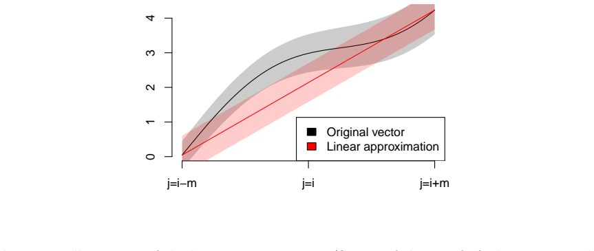
The load-bearing tool is a breakpoint lemma: if the means and variances are nearly constant on a window of length $2m$ around index $i$, then the probability that isotonic regression creates a block boundary at $i$ is at most $C(\log m)/m$. This is proved using the min-max formula for the isotonic projection, the pool-adjacent-violators truncation properties, and a classical result on the number of constant blocks in isotonic regression of standard Gaussian noise. The upper-bound proof then works in three steps: couple the noise to a Gaussian with the same means and variances; truncate to a subvector of length roughly $n^{2/3}$ centered at $i$; and compare with a linearly increasing, constant-variance subproblem whose midpoint bias is zero by symmetry. Smoothness controls the error of the linear approximation, while the breakpoint lemma controls how often truncation changes the estimate.
What would settle it
Take a strictly increasing smooth mean such as $\mu_i=i/n$, add i.i.d. Gaussian noise, and estimate $\mathbb{E}[\mathrm{iso}(Y)_{n/2}]$ by Monte Carlo for $n=1000,10000,100000$. The theorem predicts the absolute bias at this interior point decays like $n^{-2/3}$ up to logs, so a log-log regression of $|\text{bias}|$ on $n$ should have slope near $-2/3$; observing a slope near $-1/2$ or no decay would contradict the claimed sharp rate.
Extended reading notes
Core claim
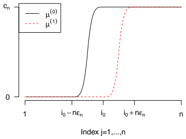
The paper establishes that when observations satisfy independent subexponential noise and the mean is Lipschitz, strictly increasing, and $(\beta,M)$-Hölder smooth, the isotonic projection $\hat{\mu}=\mathrm{iso}(Y)$ obeys $|\mathbb{E}[\hat{\mu}_i]-\mu_i| \le C(\log n/n)^{\beta/3}$ for $1\le \beta<2$ and $\le C((\log n)^5/n)^{2/3}$ for $\beta=2$, for all interior indices bounded away from the endpoints. A matching lower bound constructs means satisfying the same assumptions for which at least a constant fraction of indices have bias at least $C' n^{-\beta/3}(\log n)^{-5\beta/3}$, showing the exponent $\beta/3$ is tight up to logarithmic factors. A further result shows that if the mean is merely nondecreasing and is flat at one point, the bias can be as large as $n^{-\alpha/(2\alpha+1)}$ up to logs, which approaches $n^{-1/2}$ as $\alpha\to\infty$; strict monotonicity is therefore essential to the fast rate.
Load-bearing premise
The paper's rate relies on the mean being strictly increasing everywhere, with a positive minimum step between adjacent values; if the mean is merely nondecreasing and flattens at one point, the bias can be much larger.
Editorial extensions
If this is right
- For smooth strictly increasing signals, bias decays as $n^{-2/3}$ up to logs while the stochastic error is of order $n^{-1/3}$, so the bias is asymptotically negligible relative to the noise.
- For merely Lipschitz signals, the bias can be of order $n^{-1/3}$, the same size as the error, so the estimator can be systematically miscentered unless smoothness is assumed.
- The $n^{-\beta/3}$ rate is tight for every $\beta\in[1,2]$ up to logs, meaning no strictly increasing smoothness class with exponent $\beta$ can guarantee a faster interior bias rate in the worst case.
- The older $n^{-1/2}$ bias bound under constant variance is not the general picture: with nonconstant subexponential noise the worst-case bias is slower, and the present bounds do not require constant variance.
- Strict monotonicity is necessary for the fast rate: a flat point in an otherwise nondecreasing signal can push the bias up to $n^{-\alpha/(2\alpha+1)}$, which for smooth flat signals is $n^{-2/5}$, much larger than the strict-case $n^{-2/3}$.
Reading between the lines
- If the bias for smooth strictly increasing signals is really $O(n^{-2/3}\mathrm{polylog})$, then debiasing isotonic regression may be unnecessary for such signals: the dominant error is stochastic, and standard error-based confidence intervals could be correctly centered.
- The same combination of a breakpoint lemma and a local linear approximation may transfer to related shape-constrained estimators such as the Grenander estimator of a monotone density, where the analogous bias-variance split is still open.
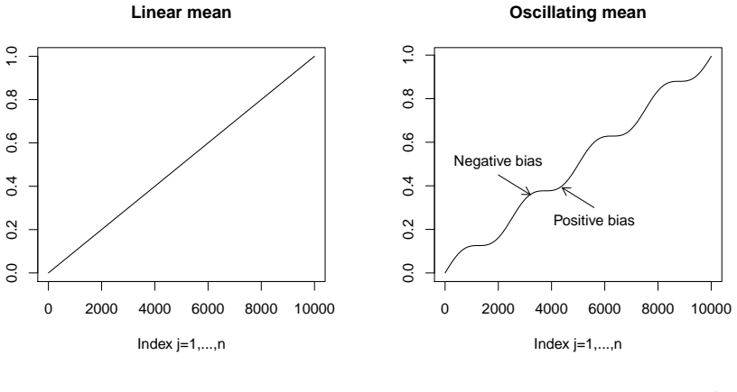
- The lower-bound construction with a linear mean plus a high-frequency sine oscillation suggests a concrete diagnostic: fit isotonic regression on a smooth increasing trend with a small superimposed oscillation and measure bias at the oscillation peaks; it should scale as the amplitude $n^{-\beta/3}$.
- For non-Gaussian noise with $\beta=2$, the paper's bound carries an extra $\log^5 n$ factor that it calls likely an artifact; a sharper proof removing it may be testable by simulation with subexponential non-Gaussian noise.
Signed reviews
Editorial analysis
A structured set of objections, weighed in public.
Referee Report
Summary. The paper studies the bias of the least-squares isotonic regression estimator for a monotone mean vector. Under a Lipschitz assumption (5), strict monotonicity (6), Hölder smoothness (7), subexponential noise (9), and a lower-bounded Lipschitz variance (10), Theorem 1 gives an entrywise bias bound of order (log n / n)^{β/3} for β ∈ [1,2) and ((log n)^5 / n)^{2/3} for β = 2, away from the endpoints. Theorem 2 constructs a signal satisfying the same conditions whose bias is at least a constant times n^{-β/3}(log n)^{-5β/3} on a constant fraction of indices, and Theorem 3 shows that if strict monotonicity is relaxed to monotonicity with a flat point, the worst-case bias can be as slow as n^{-α/(2α+1)}, approaching n^{-1/2}. The proofs combine Gaussian coupling via Sakhanenko, a breakpoint lemma for Gaussian isotonic regression, subvector restriction, and a linearization/symmetry step.
Significance. If correct, the paper provides a sharp characterization of the bias of one-dimensional isotonic regression: for smooth strictly increasing signals the bias vanishes relative to the n^{-1/3} estimation error, while for merely Lipschitz signals the bias can be of the same order as the error. The proof structure is attractive and largely modular, and the lower-bound constructions are natural. The paper also includes reproducible simulation code and a clear demonstration that strict monotonicity is essential. The main caveat is that the matching lower bound (Theorem 2) is not established by the proof as written because a stated parameter condition is unsatisfiable.
major comments (2)
- [Section 3.4, condition (25)] The parameter regime (25) includes the lower bound C3√(n log n) ≤ a_n. With the stated choice a_n = (L1+L0)/2, a constant independent of n, this inequality fails for all sufficiently large n for any fixed C3 > 0. The text states in Section 3.4 that the chosen parameters satisfy (25) and asserts this is trivial to verify; Section 3.4.4 then explicitly invokes (25) to certify m ≥ log n/(C2(C4)^{2/3}) and to control constants. Because the lower bound in (25) is impossible while the subsequent arguments appear to need only the upper bound a_n ≤ C4(c_n)^{3/2}/((log n)^2√n) — which is compatible with a_n constant, since c_n^{3/2}/((log n)^2√n) = (log n)^{1/2} — the proof of Theorem 2 is internally inconsistent as written. The theorem may be true after replacing (25) with the upper-bound condition, but the matching lower bound is not currently established by the text.
- [Section 3.4.4, Step 4] The final sentence of Step 4 states that the required conditions hold 'recalling condition (25), with C3 chosen to be sufficiently large and C4 sufficiently small.' This is not meaningful for C3: the impossible lower bound C3√(n log n) ≤ a_n cannot hold for any choice of C3 when a_n is constant, and the displayed inequalities in Step 4 do not otherwise involve C3. This reinforces that the parameter condition must be revised before the lower-bound claim can be accepted.
minor comments (5)
- [Abstract] The abstract states that the result 'only requires a strictly monotone mean and that the noise distribution has subexponential tails,' but Theorem 1 also assumes the Lipschitz bound (5), the Hölder smoothness condition (7), the variance lower bound, and the Lipschitz variance condition (10). Please restate the assumptions accurately.
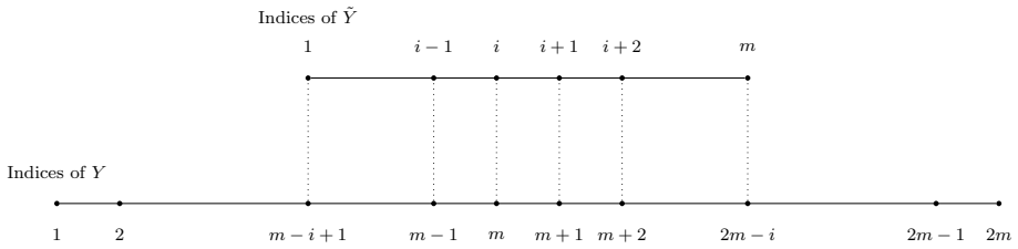
- [Lemma 3 proof] The displayed implication in the proof of Lemma 3 has the wrong direction and an invalid index: the subvector Ỹ has length m, so the expression 'iso(Ỹ)_m < iso(Ỹ)_{m+1}' is undefined. The proof should use the contrapositive of property (15) and map a break at position i in the subvector to a break at position m in the original vector; for example, with Ỹ_j = Y_{m-i+j}, the correct implication is iso(Y)_m ≠ iso(Y)_{m+1} ⇒ iso(Ỹ)_i ≠ iso(Ỹ)_{i+1}.
- [Section 3.3.3] In the paragraph introducing ˇY(i), the expression 'E[|iso(Ỹ(i))_{m+1} − iso(ˇY(i))_i|]' should read 'iso(ˇY(i))_{m+1}' rather than 'iso(ˇY(i))_i', since the subvector has length 2m+1 and its midpoint is index m+1; the subsequent equations consistently use the latter notation.
- [Section 3.4] The proof of Theorem 2 begins 'Fix any L1 > L0 ≥ 0' while the theorem statement requires L1 > L0 > 0. Please align the proof with the theorem statement.
- [Throughout] The notation '3√' for cube roots, for example in Step 2 of Section 3.3, is ambiguous in the text; using the explicit ∛{\cdot} or ∛[3]{\cdot} notation would improve readability.
Circularity Check
No significant circularity: the bias rates are derived from external coupling and breakpoint theorems, with self-citations used only as independent tools.
full rationale
The paper's derivation chain is self-contained. Theorem 1 first reduces to Gaussian noise via Sakhanenko's coupling theorem (external), then the breakpoint lemma is proved from Andersen's classical distribution of the number of blocks (Lemma 2) plus a likelihood-ratio comparison (Lemma 5). Step 3 approximates the mean by a linear vector and uses symmetry to identify zero bias in the approximating problem; the target rate emerges from the choice of block length m and the Holder exponent beta, rather than being inserted by construction. No fitted parameter is renamed as a prediction, and no known result is merely relabeled. The self-citations to Yang and Barber [2018] appear only as tools: equation (2) supplies a high-probability uniform error bound under Lipschitz and subgaussian assumptions, and their Lemma 1 is the standard 1-Lipschitz property of the isotonic projection. These results do not contain the bias rate, so they constitute independent support rather than a circular input. Theorem 2's lower bound explicitly constructs an oscillating mean and proves the bias bound through the breakpoint lemma, with bn chosen to give the desired rate; no part of the lower bound is defined in terms of the conclusion. The reviewer's concern about condition (25) in Section 3.4, where C3 sqrt(n log n) <= an fails for the chosen constant an, is a proof-gap or internal-consistency issue affecting the written justification of Theorem 2, not a circularity: it does not amount to assuming the target rate or to fitting a parameter to the predicted quantity. Overall, the central claims are not forced by definition or by a self-citation chain.
Assumptions & free parameters
assumptions (8)
- standard math Isotonic projection min-max formula and PAVA block properties (Barlow et al. (1.9), (15), (16))
- standard math Andersen's distribution of the number of blocks of isotonic regression of iid standard Gaussian noise
- standard math Sakhanenko's Gaussian coupling theorem for sums with exponential moments
- standard math Laurent-Massart chi-square concentration inequality
- standard math Yang and Barber's uniform high-probability error bound for isotonic regression
- domain assumption Strict monotonicity of means, assumption (6)
- domain assumption Hölder smoothness of means, assumption (7)
- domain assumption Subexponential tails (9) and variance conditions (10)
Cite this review
Pith. "Pith review of The bias of isotonic regression." pith.science (2026). https://pith.science/paper/XEA5DKOK
@misc{pith2026190804462,
  author       = {Pith},
  title        = {Pith review of: The bias of isotonic regression},
  year         = {2026},
  howpublished = {\url{https://pith.science/paper/XEA5DKOK}},
  note         = {Machine review of arXiv:1908.04462}
}
abstract
We study the bias of the isotonic regression estimator. While there is extensive work characterizing the mean squared error of the isotonic regression estimator, relatively little is known about the bias. In this paper, we provide a sharp characterization, proving that the bias scales as $O(n^{-\beta/3})$ up to log factors, where $1 \leq \beta \leq 2$ is the exponent corresponding to H{\"o}lder smoothness of the underlying mean. Importantly, this result only requires a strictly monotone mean and that the noise distribution has subexponential tails, without relying on symmetric noise or other restrictive assumptions.
Figures

Figures from the paper (2 more)
Reference graph
Works this paper leans on
-
[1]
E. S. Andersen. On the fluctuations of sums of random variables ii. Mathematica Scandinavica, 2: 0 194--222, Dec. 1954. doi:10.7146/math.scand.a-10407. URL https://www.mscand.dk/article/view/10407
-
[2]
M. Banerjee, C. Durot, and B. Sen. Divide and conquer in nonstandard problems and the super-efficiency phenomenon. Ann. Statist., 47 0 (2): 0 720--757, 2019. ISSN 0090-5364. doi:10.1214/17-AOS1633. URL https://doi.org/10.1214/17-AOS1633
-
[3]
R. E. Barlow, D. J. Bartholomew, J. Bremner, and H. Brunk. Statistical inference under order restrictions: The theory and application of isotonic regression. Wiley New York, 1972
work page 1972
-
[4]
D. J. Bartholomew. A test for homogeneity for ordered alternatives. Biometrika, 46: 0 36--48, 1959a
-
[5]
D. J. Bartholomew. A test for homogeneity for ordered alternatives ii. Biometrika, 46: 0 328--335, 1959b
-
[6]
H. D. Brunk. Maximum likelihood estimates of monotone parameters. Annals of Mathematical Statistics, 26: 0 607--616, 1955
work page 1955
-
[7]
H. D. Brunk. Estimation of isotonic regression. In Nonparametric T echniques in S tatistical I nference ( P roc. S ympos., I ndiana U niv., B loomington, I nd., 1969) , pages 177--197. Cambridge Univ. Press, London, 1970
work page 1969
-
[8]
E. Cator. Adaptivity and optimality of the monotone least-squares estimator. Bernoulli, 17 0 (2): 0 714--735, 05 2011. doi:10.3150/10-BEJ289. URL https://doi.org/10.3150/10-BEJ289
Show all 22 references
-
[9]
Chatterjee, A
S. Chatterjee, A. Guntuboyina, and B. Sen. On risk bounds in isotonic and other shape restricted regression problems. The Annals of Statistics, 43: 0 1774--1800, 08 2015. doi:10.1214/15-AOS1324
2015 doi
-
[10]
de Leeuw, K
J. de Leeuw, K. Hornik, and P. Mair. Isotone optimization in r: Pool-adjacent-violators (pava) and active set methods. Journal of Statistical Software, 32: 0 1--24, 2009
2009
-
[11]
C. Durot. Sharp asymptotics for isotonic regression. Probability Theory and Related Fields, 122 0 (2): 0 222--240, Feb 2002. ISSN 1432-2064. doi:10.1007/s004400100171. URL https://doi.org/10.1007/s004400100171
2002 doi
-
[12]
Durot, V
C. Durot, V. N. Kulikov, and H. P. Lopuha \"a . The limit distribution of the l_ -error of grenander-type estimators. Ann. Statist., 40 0 (3): 0 1578--1608, 06 2012. doi:10.1214/12-AOS1015. URL https://doi.org/10.1214/12-AOS1015
2012 doi
-
[13]
C. Gao, F. Han, and C.-H. Zhang. On estimation of isotonic piecewise constant signals. arXiv preprint arXiv:1705.06386, 2017
2017 arXiv
-
[14]
Grenander
U. Grenander. On the theory of mortality measurement: part ii. Scandinavian Actuarial Journal, 1956 0 (2): 0 125--153, 1956
1956
-
[15]
Guntuboyina and B
A. Guntuboyina and B. Sen. Nonparametric shape-restricted regression. Statistical Science, 33: 0 568--594, 2018
2018
-
[16]
Q. Han, T. Wang, S. Chatterjee, and R. J. Samworth. Isotonic regression in general dimensions. ArXiv e-prints, 2017
2017
-
[17]
Laurent and P
B. Laurent and P. Massart. Adaptive estimation of a quadratic functional by model selection. Annals of Statistics, pages 1302--1338, 2000
2000
-
[18]
R. E. Miles. The complete amalgamation into blocks, by weighted means, of a finite set of real numbers. Biometrika, 46: 0 317--327, 1959
1959
-
[19]
Robertson, F
T. Robertson, F. Wright, and R. Dykstra. Order Restricted Statistical Inference. Probability and Statistics Series. Wiley, 1988. ISBN 9780471917878. URL https://books.google.com/books?id=sqZfQgAACAAJ
1988
-
[20]
A. I. Sakhanenko. Convergence rate in the invariance principle for non-identically distributed variables with exponential moments. Advances in Probability Theory: Limit Theorems for Sums of Random Variables, pages 2--73, 1985
1985
-
[21]
F. T. Wright. The asymptotic behavior of monotone regression estimates. Ann. Statist., 9 0 (2): 0 443--448, 1981. ISSN 0090-5364
1981
-
[22]
Yang and R
F. Yang and R. F. Barber. Contraction and uniform convergence of isotonic regression. ArXiv e-prints, 2018
2018
Reviewed August 14, 2026 · model on record in the stance chip above.
Discussion (0). Continue with ORCID to comment.