REVIEW 5 major objections 5 minor 41 references
Graph Disentangle Causal Model: Enhancing Causal Inference in Networked Observational Data
T0 review · 5 major / 5 minor · reviewed 2026-08-11 · deepseek-v4-flash
Pith's one-line read Separating each unit's features into adjustment and confounder representations, then aggregating each separately over the graph, yields lower PEHE and ATE than treating all features as confounders on the BlogCatalog and Flickr benchmarks.
desk verdict The architecture is genuinely novel and the ablation supports the design, but the paper's headline claim of superior PEHE on both datasets is contradicted by its own Table 1 on Flickr. read the letter →
The pith
A machine-rendered reading of the paper's core claim, the machinery that carries it, and where it could break.
The reading
What carries the argument
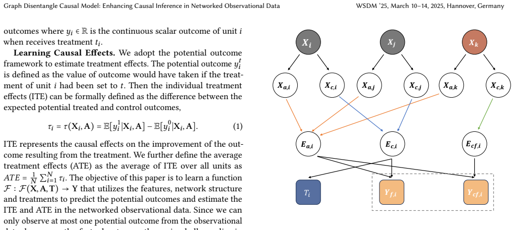
The machinery is a causal disentangle module plus targeted graph aggregation. A feature-wise mask (an element-wise gating of the feature embedding by complementary sigmoid outputs) splits $X$ into $X_c$ and $X_a$ with $X_c+X_a=X$. Three graph aggregators then form $E_a$ (adjustment, attention-weighted over all neighbors), $E_c$ (confounder, aggregated over same-treatment neighbors), and $E_{cf}$ (counterfactual confounder, aggregated over opposite-treatment neighbors), using adjustment-based attention for all three. A causal constraint module ties these to the causal graph through Eq. (19): Wasserstein-1 distance on adjustment distributions, cross-entropy treatment prediction from the confounder, mean-squared-error matching of the learned mapping $g(X_c,E_a)$ to $E_{cf}$, and a factual outcome loss. The mapping $g$ is what lets the model approximate counterfactual confounders even when a node has no opposite-treatment neighbors.
What would settle it
Build a networked dataset with a known ground-truth split—some features generated to affect only the outcome and others to affect treatment and outcome—then check whether GDC's learned masks align with the true split. If the masks do not recover the partition, or if removing all opposite-treatment edges does not change the claimed PEHE gains, the central claim is falsified.
Extended reading notes
Core claim
GDC's central claim is that the feature vector of each unit can be decomposed into two latent parts: adjustment variables, which influence only the outcome, and confounders, which influence both treatment and outcome, and that this decomposition should drive how network information is aggregated. In the model, an instance-guided sigmoid mask produces complementary adjustment and confounder features; three graph aggregators then produce an aggregated adjustment embedding, an aggregated confounder embedding from same-treatment neighbors, and an aggregated counterfactual confounder embedding from opposite-treatment neighbors, with all attention weights computed from adjustment representations because those are unbiased by treatment. A set of causal constraints—Wasserstein balance on the adjustment, treatment prediction from the confounder, a learned mapping from self-confounder and adjustment to the counterfactual confounder, and factual outcome regression—are optimized together to keep the disentangled factors faithful to the causal graph. The paper claims this design yields the best PEHE and ATE on both datasets and all values of $\kappa$, and the t-SNE visualization is offered as evidence that confounder and counterfactual confounder distributions overlap while adjustment distributions mix.
Load-bearing premise
The load-bearing premise is that the feature-wise mask and the causal constraint losses recover the true adjustment/confounder decomposition; if the mask only captures arbitrary feature variance, the counterfactual aggregation is not guaranteed to reduce confounding bias.
Editorial extensions
If this is right
- If the disentanglement is correct, forcing global balance on all features is not just unnecessary but harmful; only adjustment variables should be balanced, while confounders keep their treatment-dependent structure.
- Borrowing the confounders of opposite-treatment neighbors as counterfactual approximations gives a way to reduce confounding bias that does not require overlap in the feature space.
- Using adjustment-based attention for all three aggregators provides a treatment-unbiased similarity measure, which should make aggregation stable even under heavy treatment imbalance.
- The reported results imply that a disentangle-then-aggregate pipeline can outperform both graph-free representation balancing and single-representation graph methods on networked causal benchmarks.
- Ablations imply that both the disentangle module and the confounder pathway contribute: removing the module or using only adjustment representations degrades PEHE and ATE.
Reading between the lines
- A natural extension the paper does not test is whether the same mask-plus-constraint recipe transfers to other networked decision problems, such as uplift modeling for recommendations, where the adjustment/confounder split may be defined by a known business mechanism.
- The counterfactual confounder aggregation is only useful when enough opposite-treatment neighbors exist; a testable implication is that GDC's advantage over baselines should shrink as cross-treatment edge density decreases, since the mapping $g$ would have to carry the whole burden.
- The paper's empirical support comes from semi-synthetic graphs whose confounders are generated from neighbor topics; on graphs where confounding is not aligned with network structure, the targeted aggregation may add noise rather than remove bias.
- One could test identifiability directly by constructing data with known factors and checking whether the learned mask recovers the true partition; the paper does not provide such a check.
Editorial analysis
A structured set of objections, weighed in public.
Referee Report
Summary. The manuscript proposes GDC, a graph neural network method for estimating individual treatment effects (ITE) from networked observational data. The method disentangles each unit's features into adjustment and confounder representations via a feature-wise mask, aggregates them with three distinct graph attention operators to obtain adjustment, confounder, and counterfactual confounder embeddings, and trains with a composite loss containing prediction, adjustment-balance, treatment-prediction, and counterfactual-confonder-mapping terms. Experiments on semi-synthetic BlogCatalog and Flickr datasets compare GDC with eleven baselines and report PEHE and ATE. The central claim is that GDC achieves superior PEHE and ATE on both datasets compared with all baselines.
Significance. If the empirical and theoretical claims are established, the paper would make a useful contribution to causal inference on networked data by arguing that adjustment variables and confounders should be treated differently during graph aggregation and by introducing a counterfactual confounder aggregation and mapping mechanism. The paper is clearly written and the design is motivated by an explicit causal graph. The ablation study and hyperparameter sensitivity analysis provide useful evidence about the contribution of the main components. However, the headline performance claim is not supported by the reported table in several configurations, and the method section contains a technical inconsistency in the definition of the attention weights. The manuscript has no machine-checked proofs or released code, and the empirical support is weakened by missing variability measures and by reuse of baseline numbers from a prior paper.
major comments (5)
- [Section 3.2.1 (Eqs. 7-8)] Equations (7) and (8) are mutually recursive as written: Eq. (7) defines the aggregated adjustment embedding E_{a,i} as a function of attention coefficients alpha_{ij}, while Eq. (8) defines alpha_{ij} as a function of E_{a,i} and E_{a,j}. No initialization or fixed-point iteration is specified, so the aggregation step is not well defined. This should be corrected, most likely by computing alpha from the per-node adjustment representations X_{a,i} (or an intermediate representation) instead of from the already aggregated E_{a,i}.
- [Section 4.2 (Table 1)] The statement that "GDC exhibits superior performance in terms of PEHE and ATE on both datasets" is contradicted by the PEHE columns of Table 1. On Flickr with kappa=1, both GIAL (5.317) and GNUM (5.345) achieve lower PEHE than GDC (5.351); on Flickr with kappa=2, DRCFR (7.915) beats GDC (8.287). Averaging over the three kappa values on Flickr also puts GDC's mean PEHE (5.863) above DRCFR's (5.767). The authors should either correct the claim to reflect the actual comparison or provide additional evidence supporting a more nuanced conclusion.
- [Section 4.1.4 (Table 1)] The paper reports only the average result over ten simulations per dataset and gives no standard deviation, confidence interval, or significance test. Several reported differences are small (for example, Flickr kappa=1: GDC 5.351 versus GIAL 5.317), and without variability measures it is impossible to tell whether the remaining wins are statistically meaningful. The authors should report standard deviations or confidence intervals and, where appropriate, a paired significance test across the ten simulation runs.
- [Section 4.2] The authors state that "partial results of the baselines" are obtained from the prior paper [4] because the datasets and settings are aligned. This is not a fully controlled comparison: GDC is evaluated under the authors' current protocol, while some baseline numbers come from a different paper that may use different implementations, preprocessing, random splits, or tuning. Given that the headline claim depends on small margins, all baselines should be rerun under the same protocol, or the provenance and limitations of the copied numbers should be stated more prominently.
- [Section 3.1 / Section 3.3] The paper assumes that X can be decomposed into adjustment and confounder latent variables and then asserts that the causal constraint losses in Eq. (19) "ensure the disentangled representations as true causal factors." No identifiability argument or formal condition is provided. The feature-wise mask plus the distributional and predictive losses could select representations that satisfy the training objectives without recovering the true causal factors, in which case the counterfactual aggregation and outcome prediction in Eqs. (15)-(16) would still be biased. The authors should provide an identification condition or at least a controlled sanity check with synthetic data where the true adjustment/confounder split is known.
minor comments (5)
- [Introduction] The word "identifing" in the second paragraph should be "identifying".
- [Section 3.2.1] In the text following Eq. (7), the sentence "and E_{a,j} is the adjustment representation of unit i" appears to be a typo; it should refer to X_{a,j} or to unit j.
- [Section 4.5] The t-SNE visualizations are qualitative and do not by themselves demonstrate that the confounder and counterfactual confounder distributions coincide. Reporting a quantitative distributional discrepancy, such as the Wasserstein distance between E_c | T=t and E_cf | T != t, would strengthen the claim.
- [Section 5 / References] In the Related Work section, the reference to DRCFR is given as [13], but the paper titled "Learning Disentangled Representations for CounterFactual Regression" is reference [14]; reference [13] is a different paper on importance sampling weights.
- [Section 3.3] The counterfactual confounder mapping loss in Eq. (14) is only applied when a unit has opposite-treatment neighbors, but the mapping function g is also used in Eq. (16) for the counterfactual prediction. The training and inference behavior for units with no opposite-treatment neighbors should be clarified.
Circularity Check
No significant circularity: GDC is a learning architecture whose losses enforce its causal assumptions rather than fitting the evaluation metrics, and its self-citations are motivational only.
full rationale
GDC's derivation is self-contained as an empirical learning method. The causal disentangle module (Eqs. 2-6) is a trainable feature-wise mask; the aggregation module (Eqs. 7-10) and causal constraint losses (Eqs. 12-14, 18-19) are objectives designed to match the assumed causal graph, not quantities derived from the evaluation metrics. L_prediction uses observed factual outcomes, while PEHE/ATE are computed from held-out semi-synthetic ground truth, so no fitted parameter is renamed as a prediction. The decomposition assumption in Section 3.1 is an unproven identifiability assumption and hence a correctness risk, but it is not circular: the paper does not define the target ITE in terms of the mask or the losses. Self-citations [1, 7, 17, 34] appear only as general motivation in the introduction and related work and are not load-bearing for the architecture or the empirical claim. One empirical concern does not touch circularity: Section 4.2 borrows partial baseline numbers from [4], and the Table 1 numbers do not uniformly support the sentence claiming superiority on both datasets (e.g., Flickr kappa=1: GIAL 5.317 and GNUM 5.345 vs GDC 5.351 in PEHE; Flickr kappa=2: DRCFR 7.915 vs GDC 8.287). That is a correctness and verifiability issue, not a reduction of the result to its own inputs.
Assumptions & free parameters
free parameters (6)
- Loss weight W1 (adjustment balance) =
0.0001 (best on BlogCatalog kappa=2)
- Loss weight W2 (confounder treatment prediction) =
0.01
- Loss weight W3 (counterfactual confounder mapping) =
1
- Hidden dimension D =
256
- L2 regularization coefficient =
1e-4
- Learning rate =
0.01
assumptions (4)
- domain assumption Unconfoundedness given observed features and adjacency matrix
- domain assumption Features decompose into adjustment and confounder variables
- domain assumption Homophily in network: neighbors with opposite treatment provide approximate counterfactual confounders
- ad hoc to paper The causal constraint losses make the disentangled representations identifiable as true causal factors
invented entities (1)
-
Counterfactual confounder representation E_cf
Cite this review
Pith. "Pith review of Graph Disentangle Causal Model: Enhancing Causal Inference in Networked Observational Data." pith.science (2026). https://pith.science/paper/XEMFDZMH
@misc{pith2026241203913,
  author       = {Pith},
  title        = {Pith review of: Graph Disentangle Causal Model: Enhancing Causal Inference in Networked Observational Data},
  year         = {2026},
  howpublished = {\url{https://pith.science/paper/XEMFDZMH}},
  note         = {Machine review of arXiv:2412.03913}
}
read the original abstract
Estimating individual treatment effects (ITE) from observational data is a critical task across various domains. However, many existing works on ITE estimation overlook the influence of hidden confounders, which remain unobserved at the individual unit level. To address this limitation, researchers have utilized graph neural networks to aggregate neighbors' features to capture the hidden confounders and mitigate confounding bias by minimizing the discrepancy of confounder representations between the treated and control groups. Despite the success of these approaches, practical scenarios often treat all features as confounders and involve substantial differences in feature distributions between the treated and control groups. Confusing the adjustment and confounder and enforcing strict balance on the confounder representations could potentially undermine the effectiveness of outcome prediction. To mitigate this issue, we propose a novel framework called the \textit{Graph Disentangle Causal model} (GDC) to conduct ITE estimation in the network setting. GDC utilizes a causal disentangle module to separate unit features into adjustment and confounder representations. Then we design a graph aggregation module consisting of three distinct graph aggregators to obtain adjustment, confounder, and counterfactual confounder representations. Finally, a causal constraint module is employed to enforce the disentangled representations as true causal factors. The effectiveness of our proposed method is demonstrated by conducting comprehensive experiments on two networked datasets.
Figures


Figures from the paper (2 more)


Reference graph
Works this paper leans on
-
[4]
Zhixuan Chu, Stephen L. Rathbun, and Sheng Li. 2021. Graph Infomax Adversarial Learning for Treatment Effect Estimation with Networked Observational Data. In KDD ’21: The 27th ACM SIGKDD Conference on Knowledge Discovery and Data Mining, Virtual Event, Singapore, August 14-18, 2021 , Feida Zhu, Beng Chin Ooi, and Chunyan Miao (Eds.). ACM, 176–184. https:/...
doi:10.1145/3447548 2021
-
[1]
Zhicheng An, Zhexu Gu, Li Yu, Ke Tu, Zhengwei Wu, Binbin Hu, Zhiqiang Zhang, Lihong Gu, and Jinjie Gu. 2024. DDCDR: A Disentangle-based Distillation Framework for Cross-Domain Recommendation. In SIGKDD. 4764–4773
work page 2024
-
[2]
Martín Arjovsky, Soumith Chintala, and Léon Bottou. 2017. Wasserstein GAN. CoRR abs/1701.07875 (2017). arXiv:1701.07875 http://arxiv.org/abs/1701.07875
arXiv 2017
-
[3]
Peter C Austin. 2011. An introduction to propensity score methods for reducing the effects of confounding in observational studies. Multivariate behavioral research 46, 3 (2011), 399–424
2011
-
[5]
Marco Cuturi and Arnaud Doucet. 2014. Fast computation of Wasserstein barycen- ters. In International conference on machine learning . PMLR, 685–693
work page 2014
-
[6]
Michele Jonsson Funk, Daniel Westreich, Chris Wiesen, Til Stürmer, M Alan Brookhart, and Marie Davidian. 2011. Doubly robust estimation of causal effects. American journal of epidemiology 173, 7 (2011), 761–767
2011
-
[7]
Chunjing Gan, Binbin Hu, Bo Huang, Tianyu Zhao, Yingru Lin, Wenliang Zhong, Zhiqiang Zhang, Jun Zhou, and Chuan Shi. 2023. Which Matters Most in Making Fund Investment Decisions? A Multi-granularity Graph Disentangled Learning Framework. In SIGIR. 2516–2520
work page 2023
-
[8]
Thomas A Glass, Steven N Goodman, Miguel A Hernán, and Jonathan M Samet
Show all 41 references
-
[9]
Borgwardt, Malte J
Arthur Gretton, Karsten M. Borgwardt, Malte J. Rasch, Bernhard Schölkopf, and Alexander J. Smola. 2012. A Kernel Two-Sample Test. J. Mach. Learn. Res. 13 (2012), 723–773. https://doi.org/10.5555/2503308.2188410
2012
-
[10]
Ruocheng Guo, Jundong Li, and Huan Liu. 2020. Learning Individual Causal Effects from Networked Observational Data. In WSDM ’20: The Thirteenth ACM International Conference on Web Search and Data Mining, Houston, TX, USA, February 3-7, 2020, James Caverlee, Xia (Ben) Hu, Mouni...
2020
-
[11]
Jens Hainmueller. 2012. Entropy balancing for causal effects: A multivariate reweighting method to produce balanced samples in observational studies. Polit- ical analysis 20, 1 (2012), 25–46
2012
-
[12]
Will Hamilton, Zhitao Ying, and Jure Leskovec. 2017. Inductive representation learning on large graphs. NIPS 30 (2017)
2017
-
[13]
Negar Hassanpour and Russell Greiner. 2019. CounterFactual Regression with Importance Sampling Weights. In Proceedings of the Twenty-Eighth International Joint Conference on Artificial Intelligence, IJCAI 2019, Macao, China, August 10-16, 2019, Sarit Kraus (Ed.). ijcai.org, 58...
2019 doi
-
[14]
Negar Hassanpour and Russell Greiner. 2020. Learning Disentangled Repre- sentations for CounterFactual Regression. In 8th International Conference on Learning Representations, ICLR 2020, Addis Ababa, Ethiopia, April 26-30, 2020 . OpenReview.net. https://openreview.net/forum?id...
2020
-
[15]
Jennifer L Hill. 2011. Bayesian nonparametric modeling for causal inference. Journal of Computational and Graphical Statistics 20, 1 (2011), 217–240
2011
-
[16]
Keisuke Hirano, Guido W Imbens, and Geert Ridder. 2003. Efficient estimation of average treatment effects using the estimated propensity score. Econometrica 71, 4 (2003), 1161–1189
2003
-
[17]
Binbin Hu, Zhengwei Wu, Jun Zhou, Ziqi Liu, Zhigang Huangfu, Zhiqiang Zhang, and Chaochao Chen. 2022. MERIT: Learning Multi-level Representations on Temporal Graphs.. In IJCAI. 2073–2079
2022
-
[18]
Kosuke Imai and Marc Ratkovic. 2014. Covariate balancing propensity score. Journal of the Royal Statistical Society: Series B: Statistical Methodology (2014), 243–263
2014
-
[19]
Guido W Imbens and Donald B Rubin. 2015. Causal inference in statistics, social, and biomedical sciences. Cambridge University Press
2015
-
[20]
Song Jiang and Yizhou Sun. 2022. Estimating Causal Effects on Networked Observational Data via Representation Learning. In Proceedings of the 31st ACM International Conference on Information & Knowledge Management, Atlanta, GA, USA, October 17-21, 2022 , Mohammad Al Hasan and ...
2022
-
[21]
Johansson, Uri Shalit, and David A
Fredrik D. Johansson, Uri Shalit, and David A. Sontag. 2016. Learning Rep- resentations for Counterfactual Inference. In Proceedings of the 33nd Interna- tional Conference on Machine Learning, ICML 2016, New York City, NY, USA, June 19-24, 2016 (JMLR Workshop and Conference Pr...
2016
-
[22]
Diederik P Kingma and Jimmy Ba. 2014. Adam: A method for stochastic opti- mization. arXiv preprint arXiv:1412.6980 (2014)
2014 arXiv
-
[23]
Kipf and Max Welling
Thomas N. Kipf and Max Welling. 2017. Semi-Supervised Classification with Graph Convolutional Networks. In ICLR 2017
2017
-
[24]
Kun Kuang, Peng Cui, Bo Li, Meng Jiang, Shiqiang Yang, and Fei Wang. 2017. Treatment Effect Estimation with Data-Driven Variable Decomposition. In Pro- ceedings of the Thirty-First AAAI Conference on Artificial Intelligence, February 4-9, 2017, San Francisco, California, USA ,...
2017
-
[25]
Sören R Künzel, Jasjeet S Sekhon, Peter J Bickel, and Bin Yu. 2019. Metalearners for estimating heterogeneous treatment effects using machine learning. Proceedings of the national academy of sciences 116, 10 (2019), 4156–4165
2019
-
[26]
Mooij, David A
Christos Louizos, Uri Shalit, Joris M. Mooij, David A. Sontag, Richard S. Zemel, and Max Welling. 2017. Causal Effect Inference with Deep Latent- Variable Models. In Advances in Neural Information Processing Systems 30: An- nual Conference on Neural Information Processing Syst...
2017
-
[27]
Stephen L Morgan and Christopher Winship. 2015. Counterfactuals and causal inference. Cambridge University Press
2015
-
[28]
Paul R Rosenbaum and Donald B Rubin. 1983. The central role of the propensity score in observational studies for causal effects. Biometrika 70, 1 (1983), 41–55
1983
-
[29]
Johansson, and David A
Uri Shalit, Fredrik D. Johansson, and David A. Sontag. 2017. Estimating individual treatment effect: generalization bounds and algorithms. In Proceedings of the 34th International Conference on Machine Learning, ICML 2017, Sydney, NSW, Australia, 6-11 August 2017 (Proceedings ...
2017
-
[30]
Yongduo Sui, Caizhi Tang, Zhixuan Chu, Junfeng Fang, Yuan Gao, Qing Cui, Longfei Li, Jun Zhou, and Xiang Wang. 2024. Invariant Graph Learning for Causal Effect Estimation. In Proceedings of the ACM on Web Conference 2024 . 2552–2562
2024
-
[31]
Laurens Van der Maaten and Geoffrey Hinton. 2008. Visualizing data using t-SNE. Journal of machine learning research 9, 11 (2008)
2008
-
[32]
Petar Velickovic, Guillem Cucurull, Arantxa Casanova, Adriana Romero, Pietro Liò, and Yoshua Bengio. 2018. Graph Attention Networks. In ICLR
2018
-
[33]
Stefan Wager and Susan Athey. 2018. Estimation and inference of heterogeneous treatment effects using random forests. J. Amer. Statist. Assoc. 113, 523 (2018), 1228–1242
2018
-
[34]
Yakun Wang, Daixin Wang, Hongrui Liu, Binbin Hu, Yingcui Yan, Qiyang Zhang, and Zhiqiang Zhang. 2024. Optimizing Long-tailed Link Prediction in Graph Neural Networks through Structure Representation Enhancement. In SIGKDD. 3222–3232
2024
-
[35]
Zhiqiang Wang, Qingyun She, and Junlin Zhang. 2021. MaskNet: Introducing Feature-Wise Multiplication to CTR Ranking Models by Instance-Guided Mask. CoRR abs/2102.07619 (2021). arXiv:2102.07619 https://arxiv.org/abs/2102.07619
2021 arXiv
-
[36]
Anpeng Wu, Junkun Yuan, Kun Kuang, Bo Li, Runze Wu, Qiang Zhu, Yueting Zhuang, Fei Wu, and Senior Member. [n. d.].Learning Decomposed Representations for Treatment Effect Estimation . Technical Report
-
[37]
Feng Xia, Ke Sun, Shuo Yu, Abdul Aziz, Liangtian Wan, Shirui Pan, and Huan Liu. 2021. Graph Learning: A Survey. IEEE Trans. Artif. Intell. 2, 2 (2021), 109–127. https://doi.org/10.1109/TAI.2021.3076021
2021
-
[38]
Jingsen Zhang, Xu Chen, and Wayne Xin Zhao. 2021. Causally attentive col- laborative filtering. In Proceedings of the 30th ACM International Conference on Information & Knowledge Management . 3622–3626
2021
-
[39]
Dingyuan Zhu, Daixin Wang, Zhiqiang Zhang, Kun Kuang, Yan Zhang, Yulin Kang, and Jun Zhou. 2023. Graph neural network with two uplift estimators for label-scarcity individual uplift modeling. In Proceedings of the ACM Web Conference 2023. 395–405
2023
-
[861]
https://doi.org/10.1145/3511808.3557311
-
[2013]
Annual review of public health 34 (2013), 61–75
Causal inference in public health. Annual review of public health 34 (2013), 61–75
2013
Reviewed August 11, 2026 · model on record in the stance chip above.
Discussion (0). Continue with ORCID to comment.