Performance Variation in Deep Reinforcement Learning
Pith reviewed 2026-06-28 01:56 UTC · model grok-4.3
The pith
Deep RL algorithms show large run-to-run performance variation that conventional uncertainty estimates often underreport.
A machine-rendered reading of the paper's core claim, the machinery that carries it, and where it could break.
Core claim
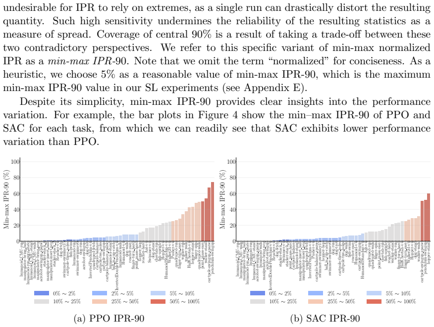
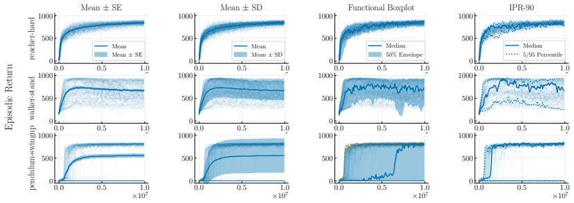
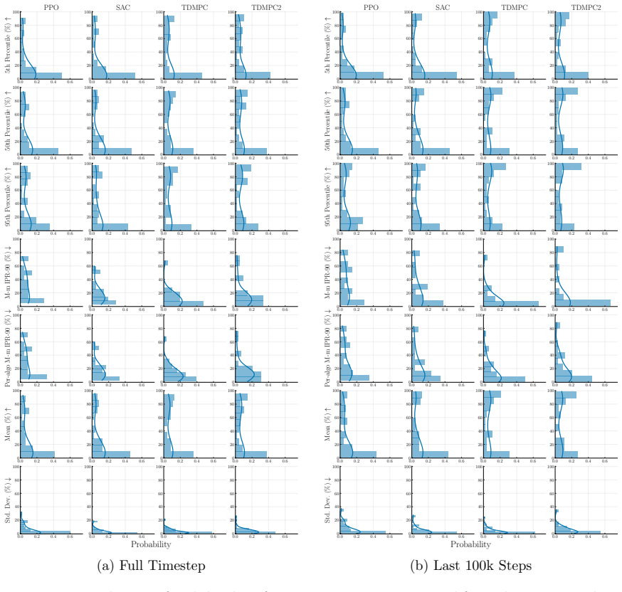
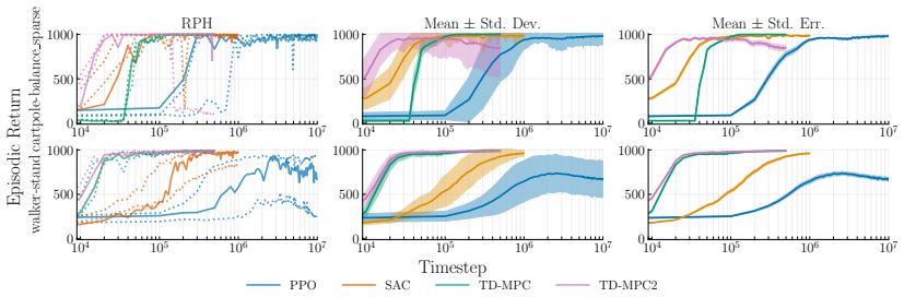
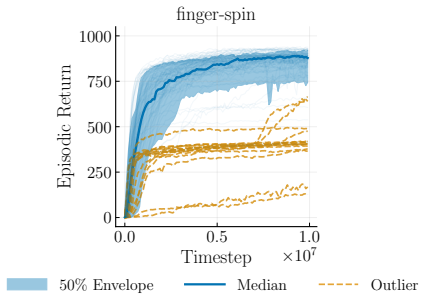
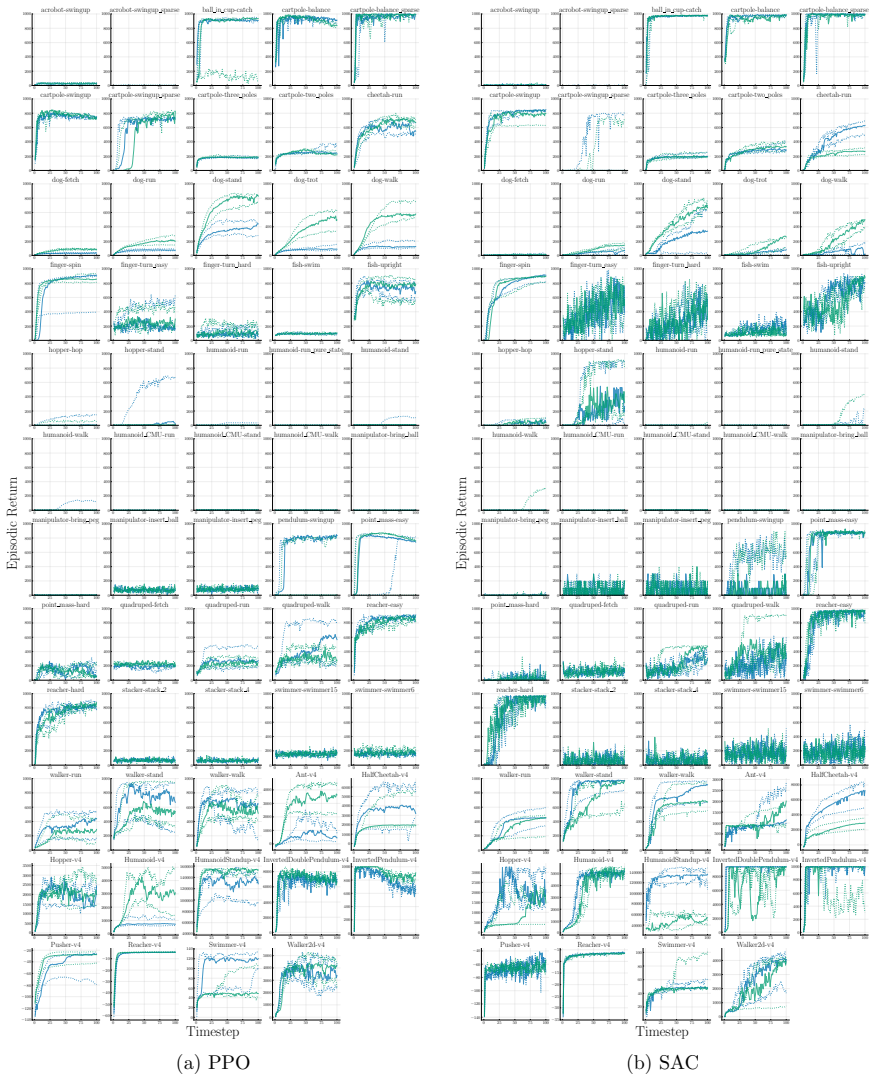
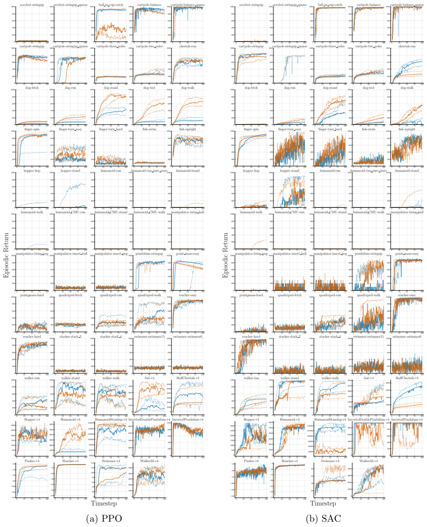
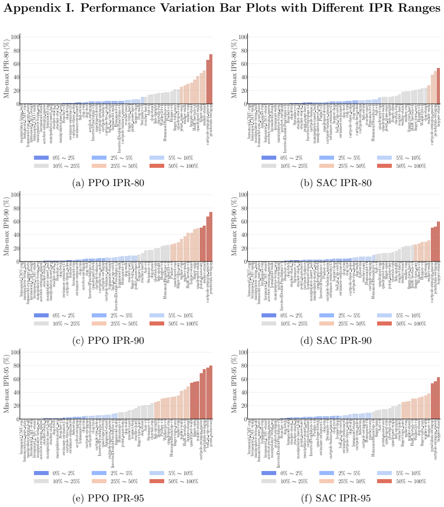
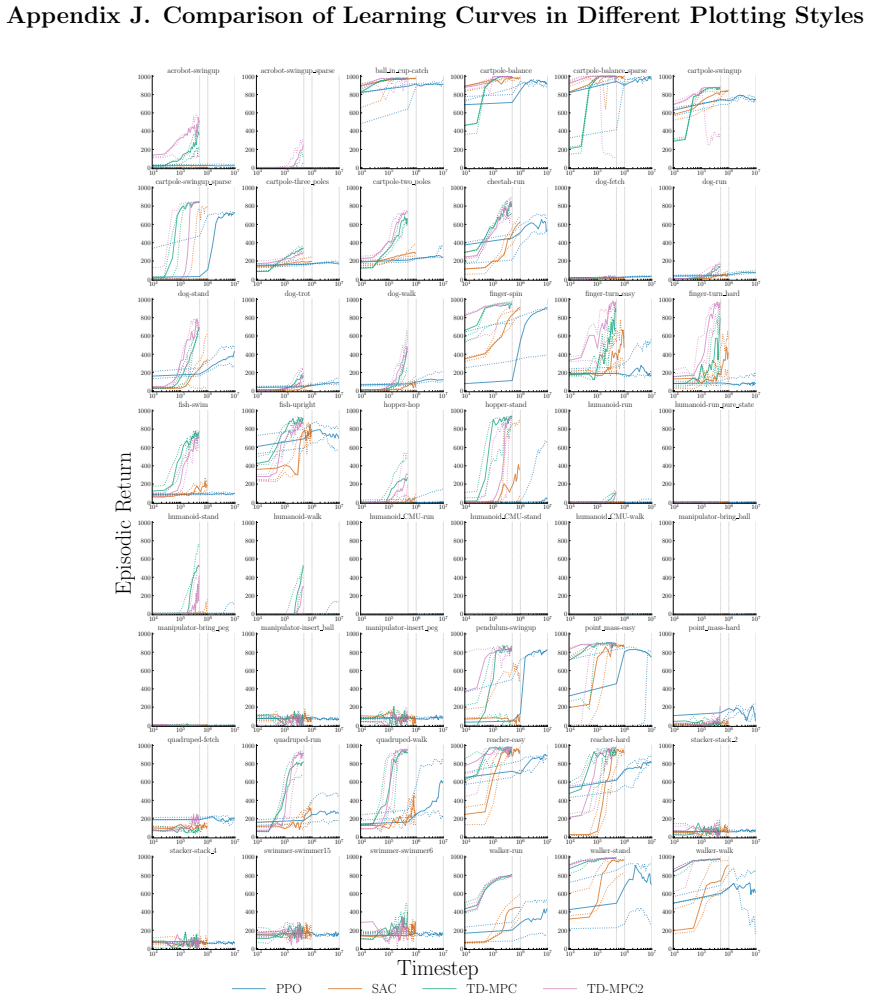
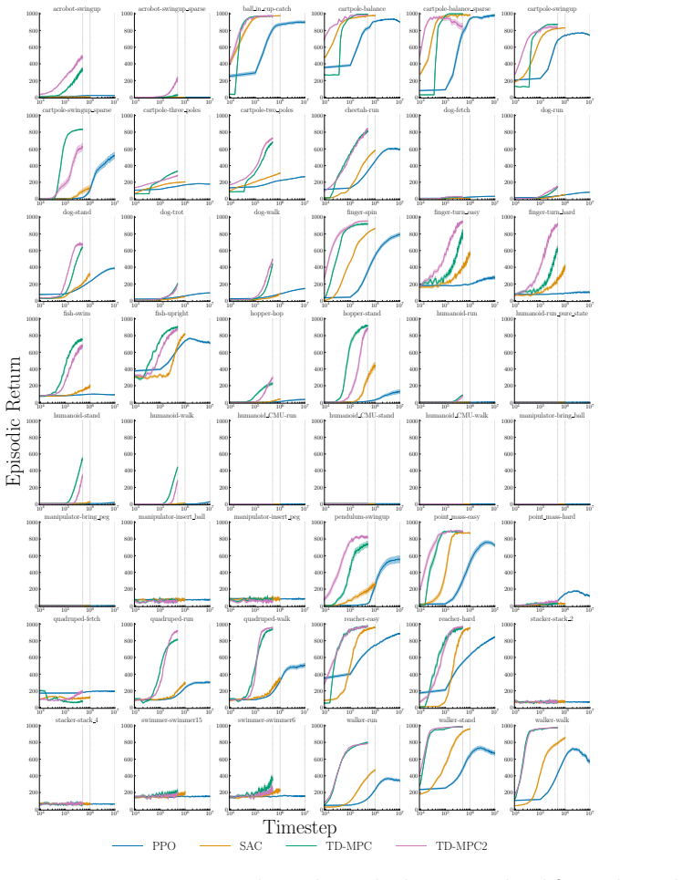
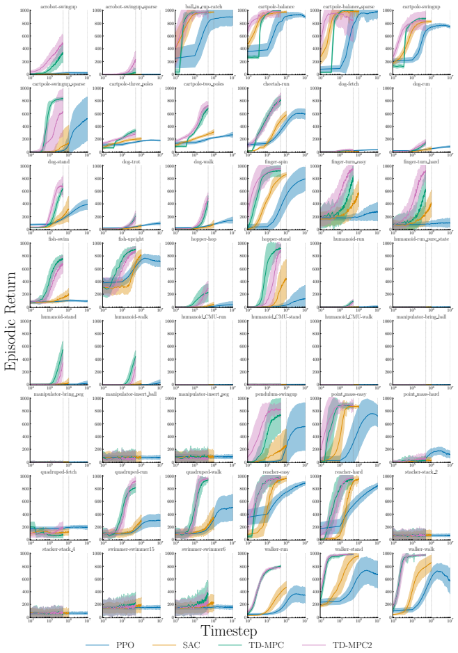
The authors claim that percentile-based tools, specifically the min-max inter-percentile range (IPR) and run-wise percentile highlighting, offer an easy-to-interpret way to quantify and visualize run-to-run performance variation in deep RL algorithms, addressing the limitations of mean-based uncertainty reporting.
What carries the argument
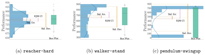
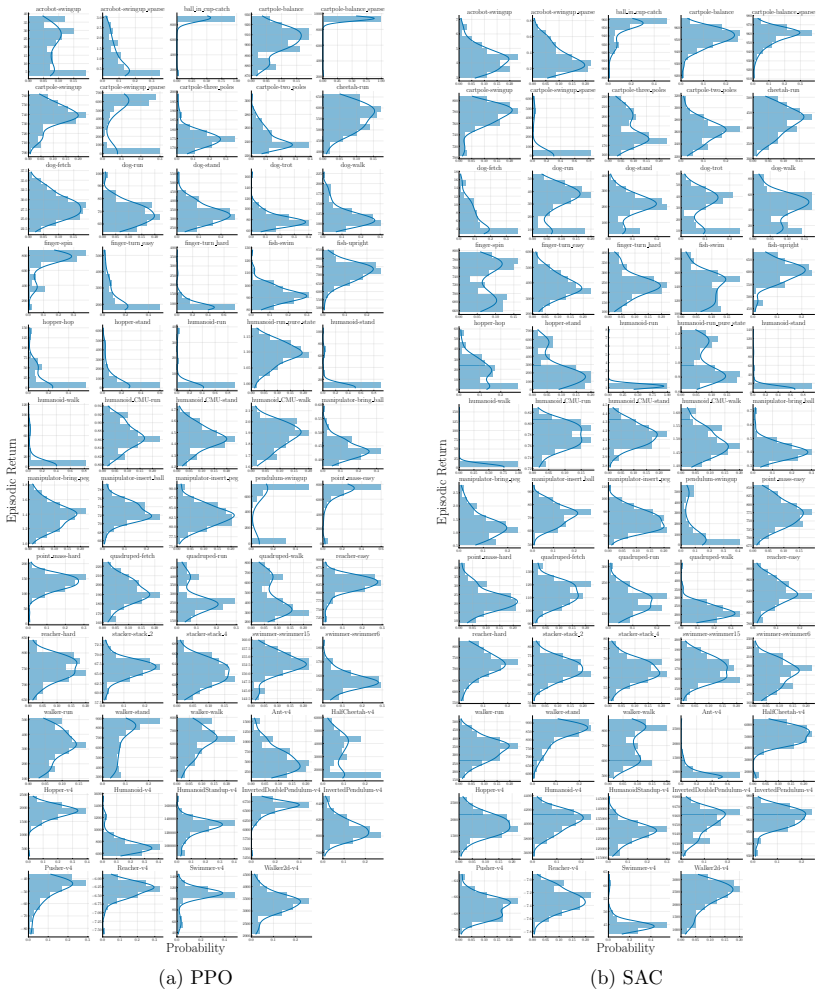
min-max IPR statistic and run-wise percentile highlighting visualization, which use sample percentiles to capture the spread of performance across multiple independent runs of the same agent configuration.
If this is right
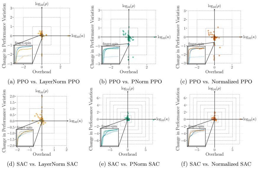
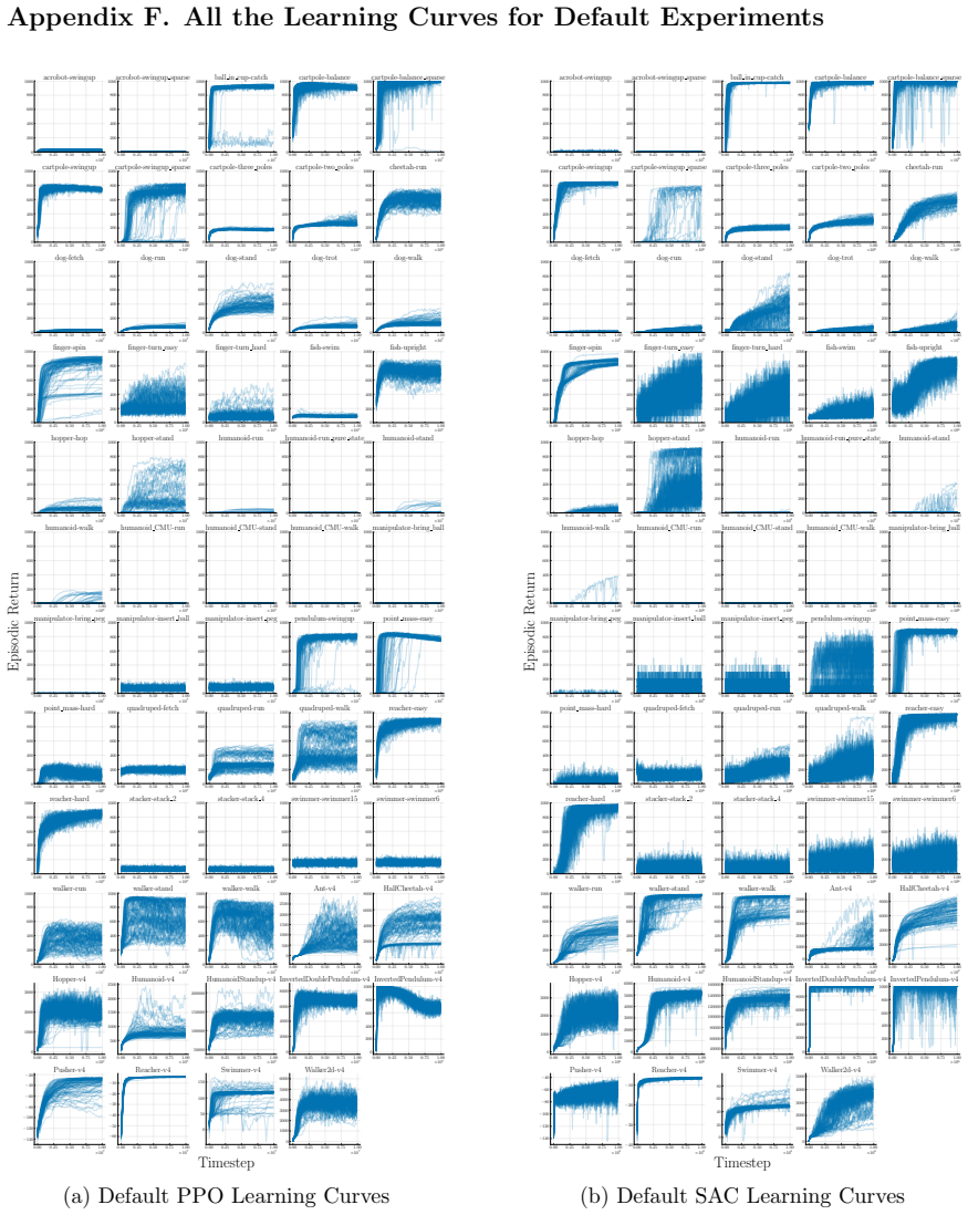
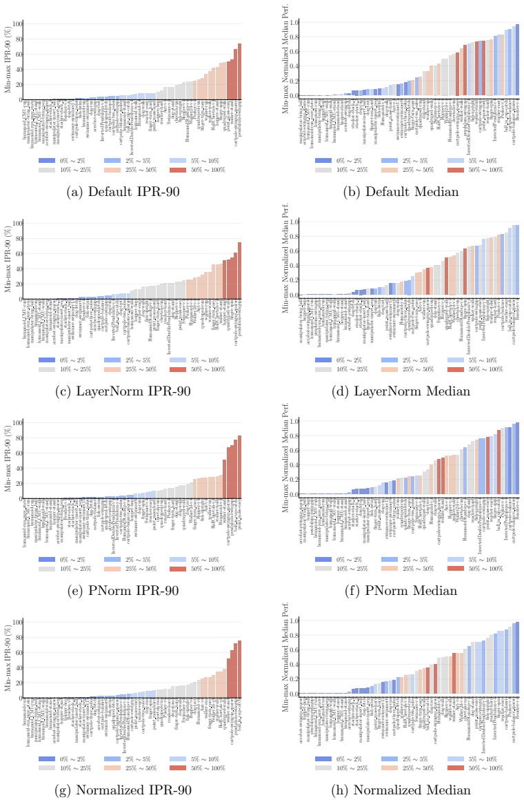
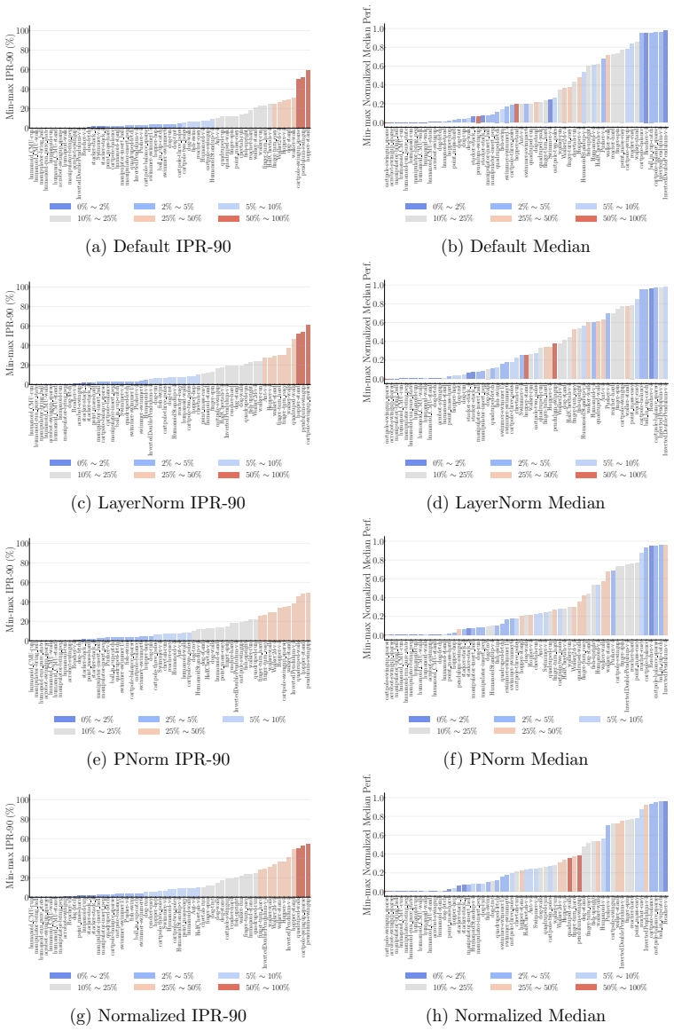
- LayerNorm and penultimate-layer normalizations narrow performance variation in PPO but leave it mostly unchanged in SAC.
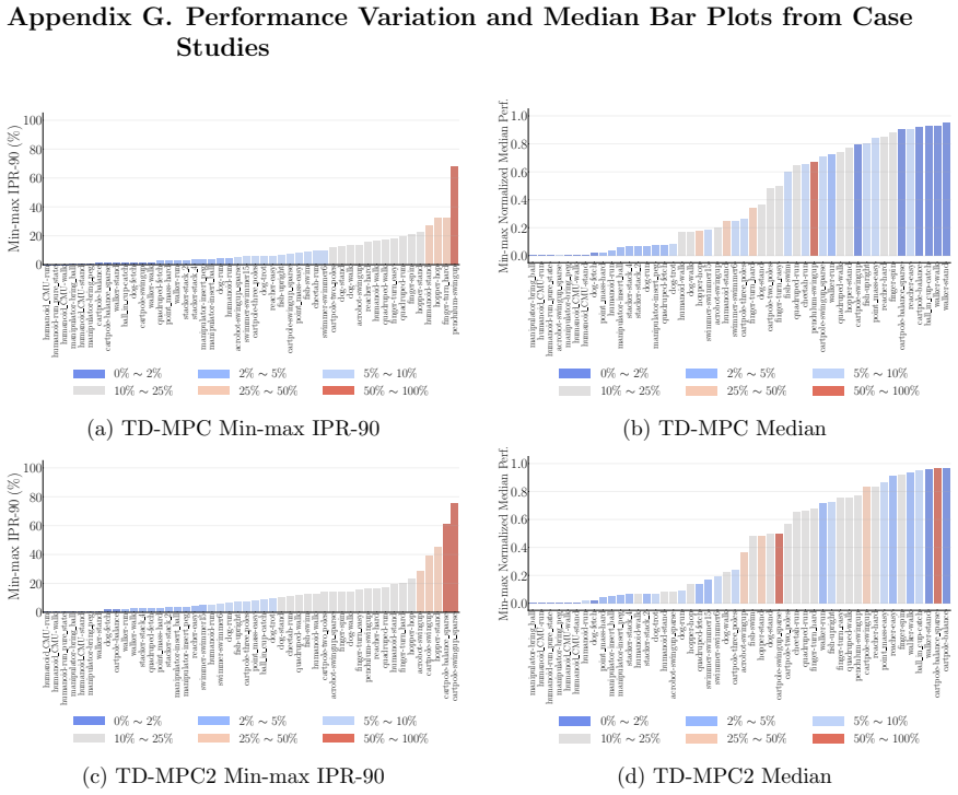
- TD-MPC exhibits the least variation while being the most data efficient among PPO, SAC, TD-MPC, and TD-MPC2.
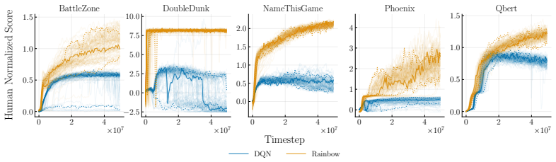
- DQN and Rainbow exhibit similar levels of performance variation on five Atari environments.
- These tools enable clearer comparisons of robustness across RL algorithms and configurations.
Where Pith is reading between the lines
- Widespread adoption could shift RL benchmark reporting toward consistent variation metrics instead of mean-focused summaries.
- The same percentile approach might apply to other machine learning areas that exhibit high run-to-run variance.
- Some reported algorithmic gains could turn out to be mainly reductions in variation rather than increases in average performance.
Load-bearing premise
Conventional uncertainty and variation estimates are misaligned with the purpose of evaluating robustness and carry a risk of underreporting variation.
What would settle it
A replication study on the same RL setups where min-max IPR and percentile highlighting yield no additional distinguishable information about run-to-run differences compared to standard deviation or confidence intervals.
Figures
read the original abstract
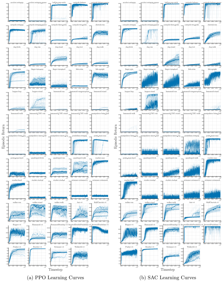
Deep reinforcement learning (RL) algorithms often suffer from low run-to-run robustness, manifesting as significant performance variation across independent runs of identically configured agents. Although this issue poses a spectrum of challenges across research and practice, relatively few studies develop methods to evaluate it; RL research instead often reports uncertainty in the estimated mean performance. In this paper, we outline the limitations of conventional uncertainty and variation estimates, particularly their misalignment with purpose and the risk of underreporting. We then propose an alternative percentile-based statistic and visualization method, min-max IPR and run-wise percentile highlighting, respectively. These percentile-based tools are easy to interpret and rely on standard properties of sample percentiles, providing rich information about run-to-run performance variation. We demonstrate this through three case studies. First, we show that LayerNorm and penultimate-layer normalizations narrow performance variation in PPO, whereas the variation is mostly unchanged in SAC. Second, we compare PPO, SAC, TD-MPC, and TD-MPC2, and show TD-MPC exhibits the least variation while being the most data efficient among the four. Finally, in a comparison of DQN and Rainbow on five Atari environments, we show that both algorithms exhibit similar levels of performance variation.
Editorial analysis
A structured set of objections, weighed in public.
Referee Report
Summary. The paper argues that conventional reporting of mean performance and uncertainty in deep RL fails to adequately capture run-to-run variation and risks underreporting robustness issues. It proposes min-max IPR (a percentile-based range statistic) and run-wise percentile highlighting visualizations as easier-to-interpret alternatives grounded in standard sample-percentile properties. These are illustrated via three case studies: effects of LayerNorm and penultimate-layer normalization on variation in PPO versus SAC; comparisons of variation and data efficiency across PPO, SAC, TD-MPC, and TD-MPC2; and performance variation in DQN versus Rainbow across five Atari environments.
Significance. If adopted, the percentile-based reporting tools could improve transparency around RL algorithm robustness without requiring new theoretical machinery, as they rest on well-understood order statistics. The case studies provide practical demonstrations on contemporary algorithms and benchmarks, highlighting differences in variation that conventional summaries might obscure. This addresses a recognized pain point in RL experimentation and could encourage more informative result presentation.
major comments (2)
- [Case studies] Case studies section: the demonstrations rely on visual inspection of the proposed visualizations and IPR values but supply no quantitative comparison (e.g., side-by-side tables of mean/std versus IPR conclusions) or statistical test showing that the new tools reduce underreporting risk relative to conventional estimates, as asserted in the introduction.
- [Introduction] Introduction: the motivation states that conventional estimates are 'misaligned with purpose' and carry underreporting risk, yet no concrete example from prior RL literature is given where mean/std reporting produced a misleading robustness conclusion that the percentile tools would have avoided.
minor comments (3)
- [Abstract] Abstract: lists the three case studies but provides no numerical findings or environment details, making it difficult to assess the scope of the empirical support at a glance.
- Notation: the exact definition of 'min-max IPR' (e.g., which percentiles define the range) should be stated explicitly in the main text with a formula, even if it follows standard practice.
- References: the manuscript would benefit from citing prior work on RL reproducibility, random seed effects, and existing variation metrics to better situate the contribution.
Simulated Author's Rebuttal
We thank the referee for the constructive review and the recommendation of minor revision. We address each major comment below, indicating where revisions will be made.
read point-by-point responses
-
Referee: [Case studies] Case studies section: the demonstrations rely on visual inspection of the proposed visualizations and IPR values but supply no quantitative comparison (e.g., side-by-side tables of mean/std versus IPR conclusions) or statistical test showing that the new tools reduce underreporting risk relative to conventional estimates, as asserted in the introduction.
Authors: We agree that side-by-side quantitative comparisons would improve clarity. In the revised manuscript we will add tables in each case study contrasting conclusions from mean/std versus min-max IPR. We do not add statistical tests, as the contribution concerns interpretability and alignment with the goal of assessing run-to-run variation rather than a claim of statistical dominance; the percentile tools rest on order statistics whose properties are already established. revision: partial
-
Referee: [Introduction] Introduction: the motivation states that conventional estimates are 'misaligned with purpose' and carry underreporting risk, yet no concrete example from prior RL literature is given where mean/std reporting produced a misleading robustness conclusion that the percentile tools would have avoided.
Authors: We acknowledge the value of a concrete prior example. However, such an example would require the raw per-run data from earlier papers, which are rarely released (only aggregate statistics appear). The three case studies in the paper serve as direct demonstrations of the misalignment. We will revise the introduction to explicitly tie the general argument to these case studies and to the known properties of sample percentiles. revision: partial
Circularity Check
No significant circularity
full rationale
The paper proposes descriptive percentile-based statistics (min-max IPR) and visualizations (run-wise percentile highlighting) for reporting run-to-run variation in RL. These rest explicitly on standard properties of sample order statistics rather than any derivation, fitted parameter, or self-referential prediction. The abstract and case-study descriptions contain no equations, no parameter estimation steps, and no load-bearing self-citations; the central claim is therefore a definitional re-description of existing statistical tools applied to RL data, with no reduction of outputs to inputs by construction.
Axiom & Free-Parameter Ledger
Forward citations
Cited by 1 Pith paper
-
Benchmarking Action Spaces in Reinforcement Learning for Vision-based Robotic Manipulation
Joint velocity action space outperforms pose increment, pose velocity, and joint position increment for smoothness and performance in sim-to-real vision-based manipulation.
Reference graph
Works this paper leans on
-
[1]
Jimmy Lei Ba, Jamie Ryan Kiros, and Geoffrey E. Hinton. Layer normalization.CoRR, abs/1607.06450,
work page internal anchor Pith review Pith/arXiv arXiv
-
[2]
Let's Play Again: Variability of Deep Reinforcement Learning Agents in Atari Environments
Kaleigh Clary, Emma Tosch, John Foley, and David Jensen. Let’s play again: Variability of deep reinforcement learning agents in atari environments.CoRR, abs/1904.06312,
work page internal anchor Pith review Pith/arXiv arXiv 1904
-
[3]
How Many Random Seeds? Statistical Power Analysis in Deep Reinforcement Learning Experiments
C´ edric Colas, Olivier Sigaud, and Pierre-Yves Oudeyer. How many random seeds? Statis- tical power analysis in deep reinforcement learning experiments.CoRR, abs/1806.08295,
work page internal anchor Pith review Pith/arXiv arXiv
- [4]
-
[5]
Proximal Policy Optimization Algorithms
John Schulman, Filip Wolski, Prafulla Dhariwal, Alec Radford, and Oleg Klimov. Proximal policy optimization algorithms.CoRR, abs/1707.06347,
work page internal anchor Pith review Pith/arXiv arXiv
-
[6]
Accelerated Methods for Deep Reinforcement Learning
Adam Stooke and Pieter Abbeel. Accelerated methods for deep reinforcement learning. CoRR, abs/1803.02811,
work page internal anchor Pith review Pith/arXiv arXiv
-
[7]
Yuval Tassa, Yotam Doron, Alistair Muldal, Tom Erez, Yazhe Li, Diego de Las Casas, David Budden, Abbas Abdolmaleki, Josh Merel, Andrew Lefrancq, Timothy Lillicrap, and Martin Riedmiller. DeepMind control suite.CoRR, abs/1801.00690,
work page internal anchor Pith review Pith/arXiv arXiv
-
[8]
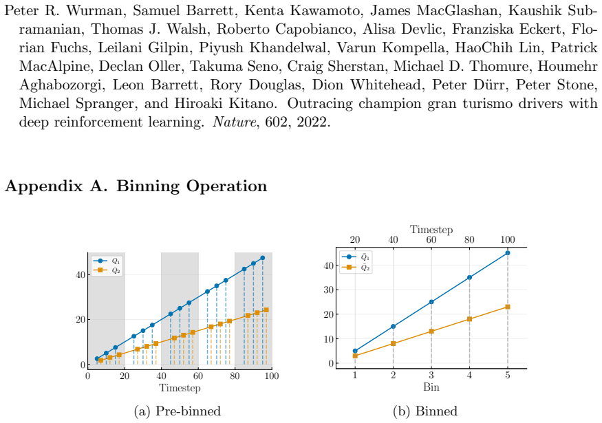
Now, consider dividing the whole timeline from 1 to 100 into 5 non-overlapping bins, as presented by the alternating shaded regions in Figure 12a
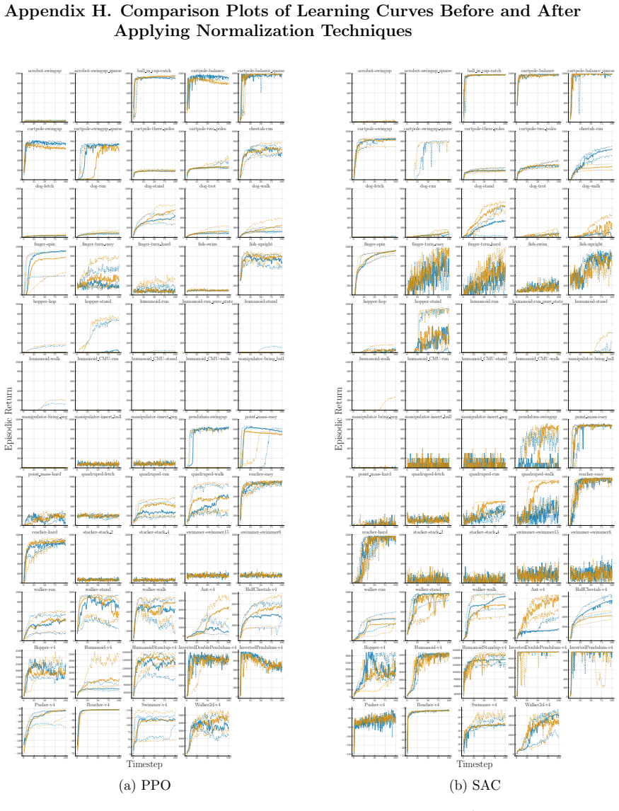
Since both timesteps of when the datapoints are collected do not align, comparing a single datapoint fromQ 1 to another inQ 2 (and vice versa) is non-trivial. Now, consider dividing the whole timeline from 1 to 100 into 5 non-overlapping bins, as presented by the alternating shaded regions in Figure 12a. By taking an average within each bin, we get ¯Q1 :=...
1968
-
[9]
Optimizer Adam Step-size 3×10 −4 27 Table 6: PPO Configurations. Parameter Configuration Total timesteps (T) 10 7 Parameter Update Frequency (B) 8192 Number of Epochs (N) 10 Minibatch Size (M) 256 Clipping Parameter (ϵ) 0.2 Value Loss Coefficient 0.5 Maximum Gradient Norm 0.5 GAEγ0.99 GAEλ0.95 Network Architecture (θ&ψ) Fully-connected NN Hidden Layer Dim...
2022
-
[10]
Hyperparameter Value Planning Horizon (H) 3 Iterations 6 (+2 if∥A∥ ≥20) Population size 512 Policy prior samples 24 Number of elites 64 Minimum std
2 Exploration Schedule (ϵ) 0.5→0.05 (25k steps) Planning Horizon Schedule 1→5 (25k steps) Batch Size 2048 (Dog) 512 (Otherwise) Momentum Coefficient (ζ) 0.99 Steps Per Gradient Update 1 θ− Update Frequency 2 29 Table 9: TD-MPC2 Hyperparameter Configurations (from Hansen et al., 2024). Hyperparameter Value Planning Horizon (H) 3 Iterations 6 (+2 if∥A∥ ≥20)...
2048
-
[11]
(ss decay)
Activation FunctionReLU Optimizer Adam Step-size 6.25×10 −5 Parameter Update Frequency 4 Minibatch Size 32 Discountγ0.99 Frequency of Target Update 10 3 Target Updateτ1.0 Sticky Action Probability 0.25 Number of Atoms 51 Minimum Value−10 Maximum Value 10 Steps forn-step Return 3 Prioritized Experience Replay (PER)α0.5 PERβ0.4 PERϵ10 −6 32 Appendix E. Supe...
2024
-
[12]
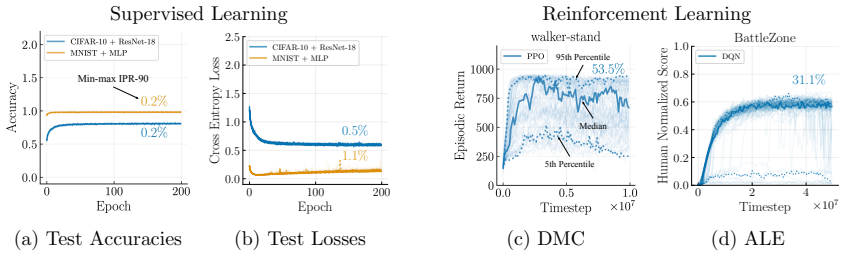
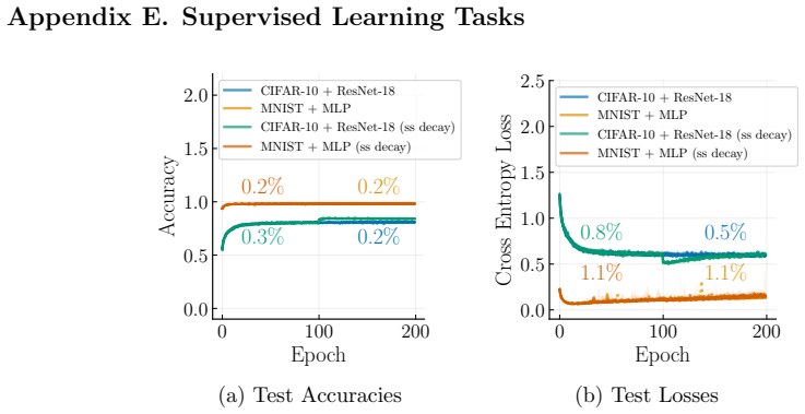
We observe that the spread in test accuracies is nearly imperceptible across all experiment configurations
Figure 14 reports test accuracies and losses over training epochs for the first two tasks in RPH format. We observe that the spread in test accuracies is nearly imperceptible across all experiment configurations. Note that the majority of the accuracy curves of each variant of the experiment overlap. Although the accuracy is wider than the test losses, th...
2000
discussion (0)
Sign in with ORCID, Apple, or X to comment. Anyone can read and Pith papers without signing in.