REVIEW 4 major objections 5 minor 42 references
VTGaussian-SLAM: RGBD SLAM for Large Scale Scenes with Splatting View-Tied 3D Gaussians
T0 review · 4 major / 5 minor · reviewed 2026-08-07 · deepseek-v4-flash
Pith's one-line read This paper claims that a 3D-Gaussian RGBD SLAM system can drop learned Gaussian positions entirely, anchoring each Gaussian to a depth pixel and learning only radius, opacity, and color, which frees memory and unlocks larger scenes.
desk verdict A clean view-tied Gaussian representation for RGBD SLAM, but the headline rendering gains largely reflect memorization of training views rather than scene quality. read the letter →
The pith
A machine-rendered reading of the paper's core claim, the machinery that carries it, and where it could break.
The reading
What carries the argument
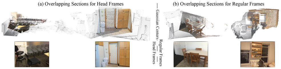
The load-bearing object is the view-tied 3D Gaussian: a spherical Gaussian whose center is the back-projection of a depth pixel through the camera pose, carrying only color, radius, and opacity as learnable attributes. Around it, the method's machinery is the section: a block of N consecutive frames whose head-frame Gaussian initialization and per-section optimization let the system keep the most relevant Gaussians learnable while freezing the rest, and whose visibility-based selection of an overlapping front section for head-frame tracking suppresses pose-error accumulation. These two mechanisms together replace the global joint optimization of all Gaussians over all keyframes that the authors identify as the scalability bottleneck of prior 3DGS SLAM.
What would settle it
Run the system on an RGBD sequence whose depth has a known artificial scale error (for example, multiply all depths by 1.02) and compare rendering PSNR and ATE against a version with untouched depth: if the biased-depth map shows a systematic geometric shift with no mechanism to correct it, the claim that frozen depth positions suffice would be put in question.
Extended reading notes
Core claim
The central claim is that Gaussian positions in RGBD SLAM can be determined entirely by the sensor depth and the camera pose, never learned. The paper's view-tied Gaussians are spheres anchored to depth pixels, so the representation stores color, radius, and opacity only, saving about 64.3% of per-Gaussian storage. Framing consecutive frames as sections, marking the first frame of each section as a head, tracking head frames against a selected overlapping previous section, and freezing all sections except the one containing the latest view removes the need for keyframe lists and for optimizing all Gaussians throughout training; the authors argue this is what allows the map to grow to much larger scenes while improving rendering quality and maintaining tracking accuracy.
Load-bearing premise
The load-bearing premise is that the sensor's depth values are an unbiased geometric prior: Gaussian centers are frozen at back-projected pixels, so any systematic depth bias or pose drift during tracking cannot be corrected by moving the map points.
Editorial extensions
If this is right
- With 5 parameters per Gaussian instead of 14, the method reports using roughly 98 million total Gaussians on Replica while keeping at most 2.7 million in GPU memory at once, so scene coverage and local detail both rise.
- Because only the section containing the latest view is optimized, the method does not need to re-render or re-optimize against a keyframe list, which the authors identify as the path to much larger scenes.
- The reported rendering gains on real indoor datasets (TUM-RGBD, ScanNet, ScanNet++) indicate that tying Gaussians to depth does not overfit a synthetic benchmark.
- On KITTI city-scale sequences in the supplementary material, the method reports markedly higher rendering PSNR and lower ATE than the same baselines, supporting the scalability claim.
Reading between the lines
- Because positions are frozen, the map inherits any systematic depth-sensor bias; a natural extension would be to learn a small per-ray offset along the projection direction while keeping position storage cheap.
- The section organization makes each local map an independent splatting unit, so merging scene parts via pose-graph registration is an obvious route to multi-session or multi-agent SLAM.
- A monocular or estimated-depth variant could inherit the same storage savings, with the frozen-position assumption tested against depth-estimation error.
- The reported tolerance to added depth noise (up to 30% of pixels) suggests the method's limit is bias rather than noise; injecting a fixed depth-scale error would pinpoint that limit.
Editorial analysis
A structured set of objections, weighed in public.
Referee Report
Summary. The paper proposes VTGaussian-SLAM, an RGBD SLAM system that represents scenes with ``view-tied 3D Gaussians''. Each Gaussian is tied to a depth pixel, so its position is determined by the back-projected depth and camera pose and is never learned; only color, radius, and opacity are optimized. The method organizes frames into sections, keeps only the current section learnable, and uses overlapping sections for tracking head frames to reduce drift. The authors claim improved rendering quality, tracking accuracy, and scalability relative to prior 3D Gaussian splatting SLAM methods, and support this with experiments on Replica, TUM-RGBD, ScanNet, ScanNet++, and KITTI, plus ablations and memory/runtime comparisons.
Significance. The view-tied representation is a simple and memory-efficient idea: reducing per-Gaussian parameters from 14 to 5 is a concrete contribution, and the section-based scheduling that avoids optimizing all Gaussians globally is a plausible mechanism for scaling to longer sequences. The paper provides extensive benchmark tables, per-scene results in the supplement, and ablations of the main design choices. However, the headline claims are not supported by the evaluation protocol. Training-view rendering metrics are reported for most benchmarks, and those metrics are structurally inflated by the fact that Gaussians are initialized at the pixels of the evaluated frames. The only held-out novel view synthesis experiment shows parity, not superiority. Tracking claims are also contradicted by the paper's own tables when prior-based methods such as LoopSplat and CG-SLAM are included. The core idea has merit, but the evidence as presented overstates the method's advantages.
major comments (4)
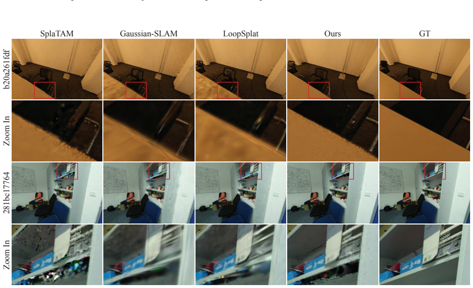
- [Sec. 4, Tab. 2, Tab. 17] The rendering evaluation is not held out. The paper states that all rendering metrics are computed by rendering full-resolution images along the estimated trajectory every 5 frames, i.e., at training views. Because Sec. 3.2 initializes a Gaussian at every pixel with valid depth using that frame's color, and Sec. 3.4 adds complement Gaussians on each regular frame, the large PSNR/SSIM/LPIPS gaps in Tab. 2 largely measure per-frame overfitting rather than scene representation quality. The only held-out test, ScanNet++ novel view synthesis (Tab. 17), shows parity: Ours 21.46 dB vs LoopSplat 21.30 dB and Gaussian-SLAM 21.27 dB. The unqualified abstract claim of ``better performance'' in rendering is therefore not supported. The authors should either report novel view synthesis results on all four benchmarks or explicitly restrict the rendering claims to training-view reconstruction and discuss why the representation does not generalize better.
- [Sec. 3.2, Sec. 3.5, Supp. D.1] The method never optimizes Gaussian positions. Sec. 3.2 freezes positions at the back-projected depth, and the bundle adjustment in Sec. 3.5 only updates the head-frame camera pose. Systematic depth bias or accumulated pose drift therefore directly enters the final map with no corrective mechanism. The noise robustness study in Supp. D.1 (Tab. 22) only adds random noise to a fraction of pixels and measures rendering PSNR/SSIM/LPIPS, not geometric accuracy; the ``movable along ray'' variant is not a full position optimization. Reconstruction F1 on Replica (Tab. 3) is 90.0, slightly below LoopSplat's 90.4, which does not demonstrate a geometry advantage. The paper should analyze the effect of biased or drifting depth on the reconstructed mesh, not just on rendered images, and should acknowledge this limitation explicitly.
- [Abstract, Sec. 4.1, Tabs. 1, 4, 5] The abstract and conclusion claim better tracking accuracy over the latest methods, but the paper's own tables show the opposite when prior-based methods are included. On Replica, Ours ATE RMSE is 0.28 cm vs LoopSplat 0.26 cm and CG-SLAM 0.27 cm (Tab. 1); on TUM-RGBD, Ours is 2.6 cm vs LoopSplat 2.3 cm and CG-SLAM 2.0 cm (Tab. 4); on ScanNet, Ours is 11.3 cm vs LoopSplat 7.7 cm and CG-SLAM 8.1 cm (Tab. 5). The text in Sec. 4.1 argues that prior-based methods are ``not a fair experimental setting,'' but this caveat does not appear in the abstract or contribution list. The tracking claim should be restricted to prior-free methods, or the comparison with prior-based methods should be discussed without claiming overall superiority.
- [Supp. B, Tabs. 20-21] The KITTI experiments used to support the large-scale claim do not state how depth maps were obtained for the RGBD SLAM pipeline. KITTI provides LiDAR point clouds but not per-frame dense aligned depth maps. Without specifying the depth generation procedure (projection, interpolation, occlusion handling, alignment to the RGB image), the large-scale results are not reproducible and the comparison with RGBD SLAM baselines is not interpretable. Please add this detail, or remove the KITTI section if the depth source is not well-defined.
minor comments (5)
- [Tab. 17] The table title contains a typo: ``Synsthesis'' should be ``Synthesis.''
- [Supp. Tab. 18] The baseline SGS-SLAM appears in the Replica rendering table but is not listed in the main text's baseline list (Sec. 4) or described in the related work; please clarify its origin and configuration.
- [Sec. 3.3] The visibility mask W_i is used in Eq. (1), but its construction is only described later in Sec. 3.3 after the optimization objective is introduced; moving the definition before Eq. (1) would improve readability.
- [Sec. 2] The phrase ``multi-view variances'' in the discussion of 3D Gaussian attributes should be ``anisotropic scales'' or ``covariances'' to use standard terminology.
- [Sec. 4, Implementation Details] The section length N is dataset-dependent (N=40 on Replica, N=30/50 on ScanNet, N=100 on ScanNet++), but the sensitivity analysis in Tab. 8 is only on Replica. A brief justification for the real-dataset choices, or an ablation on one real dataset, would strengthen the claim that the method is not heavily tuned to N.
Circularity Check
Training-view rendering advantage is a fit of per-pixel view-tied Gaussians; the only held-out novel view test shows parity.
-
fitted input called prediction
[Sec. 4 (Datasets and Metrics), with Secs. 3.2, 3.4 and Eq. 2; held-out result in Sec. C / Tab. 17]
"Sec. 4: "all the rendering metrics are computed by rendering the full resolution images along the estimated trajectory every 5 frames." Sec. 3.2: "We remove the need of learning and storing locations by tying a Gaussian g at each pixel with a valid depth value on the depth map. We center g at the 3D location back-projected from the depth value." Sec. 3.4: "we first initialize Gaussians at all pixels on the depth map at the head frame." Eq. 2 minimizes ρ||Vi − V′i||1 + τLS(Vi, V′i) + σUi||Di − D′i||1 against those observations."
The headline rendering claim (Abstract: "improving rendering quality"; Sec. 4.1: "our method produces the best rendered images, as shown in Tab. 2") is supported by metrics computed at poses on the estimated trajectory, i.e., at the same frames used during mapping. The representation is defined by tying each Gaussian to a pixel of such a frame and back-projecting it from that frame's depth and pose; the mapping step then minimizes the RGB-D residual at exactly those frames. Thus Tab. 2's PSNR/SSIM/LPIPS values are a measure of how well the model fits its own per-pixel store, not of predicted novel views. This is confirmed by the only held-out evaluation: ScanNet++ novel view synthesis (Tab. 17) gives 21.46 dB vs LoopSplat 21.30 and Gaussian-SLAM 21.27, i.e., parity.
full rationale
This paper contains no derivation chain in the usual sense; its contribution is a directly defined representation plus tracking/mapping strategies, and most claims are checked against external baselines and ablations. There is no load-bearing self-citation chain: DF-Prior (Hu & Han 2023) appears only in related work and as a baseline, and no uniqueness theorem is imported from the authors' prior work. Tracking accuracy, reconstruction F1, memory, and runtime results are measured against independent systems and are not circular. The one load-bearing circularity is the rendering-quality claim: the flagship Tab. 2 metric is computed on training frames, while Secs. 3.2 and 3.4 initialize Gaussians at exactly those frames' valid-depth pixels and Eq. 2 optimizes the same frames' RGB-D errors. Consequently the reported rendering advantage is a fitted input called a prediction, and it collapses to parity on the paper's only held-out novel-view benchmark (ScanNet++, Tab. 17). This warrants a partial-circularity score of 6 rather than a higher score because tracking, scalability, memory usage, and reconstruction remain independently evaluated. The frozen-depth bias concern noted by the reader is a robustness limitation, not a circularity.
Assumptions & free parameters
free parameters (6)
- Section length N =
40 (Replica); 30 or 50 (ScanNet); 30 (TUM-RGBD); 100 (ScanNet++)
- Tracking weights alpha and beta =
alpha=0.5; beta=0.025 (Replica), 1.0 (TUM-RGBD and ScanNet++), 0.9 (ScanNet)
- Mapping weights rho, tau, sigma =
rho=0.8, tau=0.2, sigma=1.0
- Overlap threshold gamma and coverage mask threshold =
gamma=0.26 (TUM), 0.24 (ScanNet and ScanNet++); mask threshold 0.5
- Learning rates =
color 0.0025, radius 0.005, opacity 0.05; pose lrrot and lrtrans differ per dataset
- Candidate view interval N1 =
5
assumptions (5)
- domain assumption Differentiable Gaussian splatting provides an accurate image formation model for optimization.
- domain assumption Depth maps are an unbiased geometric prior; Gaussian centers need no position optimization.
- domain assumption Local section-level optimization maintains global consistency; frozen sections remain valid.
- domain assumption Pose initialization by constant-speed assumption, or odometry on ScanNet++, is accurate enough for tracking convergence.
- domain assumption Visibility masks computed by depth interpolation and silhouette projection capture occlusions.
Cite this review
Pith. "Pith review of VTGaussian-SLAM: RGBD SLAM for Large Scale Scenes with Splatting View-Tied 3D Gaussians." pith.science (2026). https://pith.science/paper/XKQ4O3HO
@misc{pith2026250602741,
  author       = {Pith},
  title        = {Pith review of: VTGaussian-SLAM: RGBD SLAM for Large Scale Scenes with Splatting View-Tied 3D Gaussians},
  year         = {2026},
  howpublished = {\url{https://pith.science/paper/XKQ4O3HO}},
  note         = {Machine review of arXiv:2506.02741}
}
read the original abstract
Jointly estimating camera poses and mapping scenes from RGBD images is a fundamental task in simultaneous localization and mapping (SLAM). State-of-the-art methods employ 3D Gaussians to represent a scene, and render these Gaussians through splatting for higher efficiency and better rendering. However, these methods cannot scale up to extremely large scenes, due to the inefficient tracking and mapping strategies that need to optimize all 3D Gaussians in the limited GPU memories throughout the training to maintain the geometry and color consistency to previous RGBD observations. To resolve this issue, we propose novel tracking and mapping strategies to work with a novel 3D representation, dubbed view-tied 3D Gaussians, for RGBD SLAM systems. View-tied 3D Gaussians is a kind of simplified Gaussians, which is tied to depth pixels, without needing to learn locations, rotations, and multi-dimensional variances. Tying Gaussians to views not only significantly saves storage but also allows us to employ many more Gaussians to represent local details in the limited GPU memory. Moreover, our strategies remove the need of maintaining all Gaussians learnable throughout the training, while improving rendering quality, and tracking accuracy. We justify the effectiveness of these designs, and report better performance over the latest methods on the widely used benchmarks in terms of rendering and tracking accuracy and scalability. Please see our project page for code and videos at https://machineperceptionlab.github.io/VTGaussian-SLAM-Project .
Figures


Figures from the paper (14 more)






Reference graph
Works this paper leans on
-
[3]
Geiger, A., Lenz, P., and Urtasun, R
URL https: //arxiv.org/abs/2402.04796. Geiger, A., Lenz, P., and Urtasun, R. Are we ready for autonomous driving? the kitti vision benchmark suite. In Computer Vision and Pattern Recognition,
-
[5]
2d gaussian splatting for geometrically accurate radi- ance fields
Huang, B., Yu, Z., Chen, A., Geiger, A., and Gao, S. 2d gaussian splatting for geometrically accurate radi- ance fields. In SIGGRAPH 2024 Conference Papers . Association for Computing Machinery, 2024a. doi: 10.1145/3641519.3657428. Huang, H., Li, L., Hui, C., and Yeung, S.-K. Photo-slam: Real-time simultaneous localization and photorealistic mapping for m...
arXiv 2024
-
[6]
Kong, X., Liu, S., Taher, M., and Davison, A
URL https://repo-sam.inria.fr/ fungraph/3d-gaussian-splatting/. Kong, X., Liu, S., Taher, M., and Davison, A. J. vmap: Vectorised object mapping for neural field slam. arXiv preprint arXiv:2302.01838,
-
[7]
URL https://arxiv. org/abs/2402.03246. Li, Z., Lyu, X., Ding, Y ., Wang, M., Liao, Y ., and Liu, Y . Rico: Regularizing the unobservable for indoor composi- tional reconstruction,
-
[8]
URL https://arxiv. org/abs/2405.06945. Liso, L., Sandstr ¨om, E., Yugay, V ., Van Gool, L., and Os- wald, M. R. Loopy-slam: Dense neural slam with loop closures. In Proceedings of the IEEE/CVF Conference on Computer Vision and Pattern Recognition, pp. 20363– 20373,
-
[9]
Instant neural graphics primitives with a multiresolution hash encoding
M¨uller, T., Evans, A., Schied, C., and Keller, A. Instant neural graphics primitives with a multiresolution hash encoding. arXiv:2201.05989,
-
[10]
∗ indicates methods relying on pre-trained data-driven priors
Tracking performance comparisons in ATE RMSE ↓ [cm] on Replica (Straub et al., 2019). ∗ indicates methods relying on pre-trained data-driven priors. Method Rm0 Rm1 Rm2 Off0 Off1 Off2 Off3 Off4 Avg. Neural Implicit Fields NICE-SLAM (Zhu et al.,
work page 2019
-
[11]
∗ indicates methods relying on pre-trained data-driven priors
Tracking performance comparisons in ATE RMSE ↓ [cm] on TUM-RGBD (Sturm et al., 2012). ∗ indicates methods relying on pre-trained data-driven priors. Method fr1/desk fr2/xyz fr3/office Avg. Neural Implicit Fields NICE-SLAM (Zhu et al.,
work page 2012
Show all 42 references
-
[12]
org/abs/2406.04861
URL https://arxiv. org/abs/2406.04861. R¨uckert, D., Franke, L., and Stamminger, M. Adop: Approximate differentiable one-pixel point rendering. arXiv:2110.06635,
-
[13]
R., and Tombari, F
Sandstr¨om, E., Tateno, K., Oechsle, M., Niemeyer, M., Van Gool, L., Oswald, M. R., and Tombari, F. Splat- slam: Globally optimized rgb-only slam with 3d gaus- sians. arXiv preprint arXiv:2405.16544,
-
[14]
Straub, J., Whelan, T., Ma, L., Chen, Y ., Wijmans, E., Green, S., Engel, J
URL https://arxiv.org/abs/2409.02104. Straub, J., Whelan, T., Ma, L., Chen, Y ., Wijmans, E., Green, S., Engel, J. J., Mur-Artal, R., Ren, C., Verma, S., Clark- son, A., Yan, M., Budge, B., Yan, Y ., Pan, X., Yon, J., Zou, Y ., Leon, K., Carter, N., Briales, J., Gillingham, T....
1906 arXiv
-
[15]
∗ indicates methods relying on pre-trained data-driven priors
Tracking performance comparisons in ATE RMSE ↓ [cm] on ScanNet++ (Yeshwanth et al., 2023). ∗ indicates methods relying on pre-trained data-driven priors. Method a b c d e Avg. Neural Implicit Fields Point-SLAM (Sandstr¨om et al., 2023a) 246.16 632.99 830.79 271.42 574.86 511.2...
2023
-
[16]
We additionally report our performance on extremely large scenes, such as city-level scenes in KITTI (Geiger et al., 2012)
Large-scale scenes Results. We additionally report our performance on extremely large scenes, such as city-level scenes in KITTI (Geiger et al., 2012). Since many moving objects exist in KITTI sequences, we only select part of the sequences to evaluate our tracking and renderi...
2012
-
[17]
∗ indicates methods relying on pre-trained data-driven priors
Novel View Synsthesis performance comparison in PSNR ↑ on ScanNet++ (Yeshwanth et al., 2023). ∗ indicates methods relying on pre-trained data-driven priors. Method a b c d e Avg. 3D Gaussian Splatting SplaTAM (Keetha et al.,
2023
-
[18]
Wolf, Y ., Bracha, A., and Kimmel, R
URL https://arxiv.org/abs/2408.12677. Wolf, Y ., Bracha, A., and Kimmel, R. Gs2mesh: Surface reconstruction from gaussian splatting via novel stereo views. arXiv preprint arXiv:2404.01810,
-
[19]
V ox-fusion: Dense tracking and mapping with voxel-based neural implicit representation
Yang, X., Li, H., Zhai, H., Ming, Y ., Liu, Y ., and Zhang, G. V ox-fusion: Dense tracking and mapping with voxel-based neural implicit representation. In 2022 IEEE International Symposium on Mixed and Aug- mented Reality (ISMAR) , Dec
2022
-
[20]
URL http://dx.doi
doi: 10.1109/ ISMAR55827.2022.00066. URL http://dx.doi. org/10.1109/ismar55827.2022.00066. Yeshwanth, C., Liu, Y .-C., Nießner, M., and Dai, A. Scan- net++: A high-fidelity dataset of 3d indoor scenes. In Proceedings of the International Conference on Computer Vision (ICCV),
2022
-
[21]
MonoSDF: Exploring monocular geometric cues for neural implicit surface reconstruction
Yu, Z., Peng, S., Niemeyer, M., Sattler, T., and Geiger, A. MonoSDF: Exploring monocular geometric cues for neural implicit surface reconstruction. ArXiv, abs/2022.00665,
2022
-
[22]
Impact of depth noise and movability of Gaussians on the rendering performance in PSNR ↑, SSIM ↑, and LPIPS ↓ on Replica (Straub et al., 2019). Metric 10% pixels w/ noises 20% pixels w/ noises 30% pixels w/ noises Gaussians movable along ray Ours(w/o additional noises & fix) P...
2019
-
[23]
Mononeuralfusion: Online monocular neural 3d recon- struction with geometric priors
Zou, Z., Huang, S., Cao, Y ., Mu, T., Shan, Y ., and Fu, H. Mononeuralfusion: Online monocular neural 3d recon- struction with geometric priors. CoRR, abs/2209.15153,
-
[24]
Addi- tionally, we also show more results regarding Novel View Synthesis on ScanNet++ (Yeshwanth et al., 2023)
13 Supplementary Material In this supplementary material, we will cover more details about the implementation and results on each scene. Addi- tionally, we also show more results regarding Novel View Synthesis on ScanNet++ (Yeshwanth et al., 2023). A. Implementation Details We...
2023
-
[25]
to help the pose initialization if the rendering error with the pose initialized by constant speed assumption is 50 times larger than the average of the rendering loss for previous frames after the tracking optimization. We set the learning rate of pose to lrrot = 0.0004 and l...
2019
-
[26]
Please refer to our supplementary video for more details of this comparison. We also report comparisons in rendering in each scene from the training views in Replica (Straub et al., 2019), TUM- RGBD (Sturm et al., 2012), ScanNet (Dai et al., 2017a), and ScanNet++ (Yeshwanth et al.,
2019
-
[28]
We use a little bit more memory, but we manage to use more Gaussians to produce much better rendering
Each method uses the most Gaussians until no improvement can be made. We use a little bit more memory, but we manage to use more Gaussians to produce much better rendering. C. Novel View Synthesis We evaluate the performance in novel view synthesis on ScanNet++ (Yeshwanth et a...
2023
-
[31]
∗ indicates methods relying on pre-trained data-driven priors
Rendering performance comparison in PSNR ↑, SSIM ↑, and LPIPS ↓ on TUM-RGBD (Sturm et al., 2012). ∗ indicates methods relying on pre-trained data-driven priors. Method Metric fr1/desk fr2/xyz fr3/office Avg. Neural Implicit Fields NICE-SLAM (Zhu et al.,
2012
-
[33]
∗ indicates methods relying on pre-trained data-driven priors
Rendering performance comparison in PSNR ↑ on ScanNet++ (Yeshwanth et al., 2023). ∗ indicates methods relying on pre-trained data-driven priors. Method a b c d e Avg. 3D Gaussian Splatting SplaTAM (Keetha et al.,
2023
-
[35]
b20a261fdf281bc17764 Zoom In LoopSplat Ours GT Gaussian-SLAM SplaTAM Zoom In Figure
Visual comparisons in training view rendering on ScanNet++ (Yeshwanth et al., 2023). b20a261fdf281bc17764 Zoom In LoopSplat Ours GT Gaussian-SLAM SplaTAM Zoom In Figure
2023
-
[36]
20 Table
Visual comparisons in novel view rendering on ScanNet++ (Yeshwanth et al., 2023). 20 Table
2023
-
[37]
∗ indicates methods relying on pre-trained data-driven priors
Rendering performance comparisons in PSNR ↑, SSIM ↑, and LPIPS ↓ on Replica (Straub et al., 2019). ∗ indicates methods relying on pre-trained data-driven priors. Method Metric Rm0 Rm1 Rm2 Off0 Off1 Off2 Off3 Off4 Avg. Neural Implicit Fields NICE-SLAM (Zhu et al.,
2019
-
[38]
∗ indicates methods relying on pre-trained data-driven priors
Reconstruction performance comparison in Depth L1 [cm]↓ and F1 [%] ↑ on Replica (Straub et al., 2019). ∗ indicates methods relying on pre-trained data-driven priors. Method Metric Rm0 Rm1 Rm2 Off0 Off1 Off2 Off3 Off4 Avg. Neural Implicit Fields NICE-SLAM (Zhu et al.,
2019
-
[39]
Depth L1 [cm]↓ 1.31 0.82 1.26 0.81 0.96 1.41 1.53 1.08 1.16 F1 [%]↑ 62.9 79.9 66.8 80.0 81.6 66.0 59.2 65.0 70.2 Gaussian-SLAM (Yugay et al., 2023)Depth L1 [cm]↓ 0.61 0.25 0.54 0.50 0.52 0.98 1.63 0.42 0.68 F1 [%]↑ 88.8 91.4 90.5 91.7 90.1 87.3 84.2 87.4 88.9 LoopSplat∗ (Zhu et al.,
2023
-
[40]
Sequence Gaussian-SLAM SplaTAM LoopSplat Ours 00 3.02 58.83 2.22 2.06 01 77.51 84.45 74.47 29.01 05 128.88 80.39 117.43 7.74 10 10.60 43.82 11.39 4.54 Table
Tracking performance comparisons in ATE RMSE ↓ [m] on KITTI (Geiger et al., 2012). Sequence Gaussian-SLAM SplaTAM LoopSplat Ours 00 3.02 58.83 2.22 2.06 01 77.51 84.45 74.47 29.01 05 128.88 80.39 117.43 7.74 10 10.60 43.82 11.39 4.54 Table
2012
-
[41]
Rendering performance comparisons in PSNR ↑ on KITTI (Geiger et al., 2012). Sequence Gaussian-SLAM SplaTAM LoopSplat Ours 00 15.51 9.82 15.82 28.54 01 15.95 12.89 14.69 30.33 05 16.22 26.48 15.98 28.19 10 15.58 25.58 14.58 27.59 Peak GPU Use (GiB) 2.74 22.37 3.56 4.79 Table
2012
-
[2004]
doi: 10.1109/TIP.2003.819861. Wei, J. and Leutenegger, S. Gsfusion: Online rgb-d mapping where gaussian splatting meets tsdf fusion,
2003
-
[2012]
Sucar, E., Liu, S., Ortiz, J., and Davison, A
doi: 10.1109/IROS.2012.6385773. Sucar, E., Liu, S., Ortiz, J., and Davison, A. J. imap: Implicit mapping and positioning in real-time. In Proceedings of the IEEE/CVF International Conference on Computer Vision, pp. 6229–6238,
2012
-
[2017]
Park, K., Sinha, U., Barron, J
doi: 10.1109/ICCV .2017.25. Park, K., Sinha, U., Barron, J. T., Bouaziz, S., Goldman, D. B., Seitz, S. M., and Martin-Brualla, R. Nerfies: De- formable neural radiance fields. IEEE International Con- ference on Computer Vision,
2017 doi
-
[2018]
Zhang, W., Liu, Y .-S., and Han, Z
URLhttps://arxiv.org/ abs/1801.03924. Zhang, W., Liu, Y .-S., and Han, Z. Neural signed distance function inference through splatting 3d gaussians pulled on zero-level set. In Advances in Neural Information Processing Systems, 2024b. Zhang, W., Shi, K., Liu, Y .-S., and Han, Z...
-
[2019]
A benchmark for the evaluation of rgb-d slam 11 systems
Sturm, J., Engelhard, N., Endres, F., Burgard, W., and Cre- mers, D. A benchmark for the evaluation of rgb-d slam 11 systems. In 2012 IEEE/RSJ International Conference on Intelligent Robots and Systems , pp. 573–580,
2012
-
[2021]
Neural graph mapping for dense slam with efficient loop closure
Bruns, L., Zhang, J., and Jensfelt, P. Neural graph mapping for dense slam with efficient loop closure. arXiv preprint arXiv:2405.03633,
-
[2022]
Colored point cloud registration revisited
Park, J., Zhou, Q.-Y ., and Koltun, V . Colored point cloud registration revisited. In 2017 IEEE International Con- ference on Computer Vision (ICCV), pp. 143–152,
2017
-
[2023]
Cg-slam: Efficient dense rgb-d slam in a consistent uncertainty-aware 3d gaussian field
Hu, J., Chen, X., Feng, B., Li, G., Yang, L., Bao, H., Zhang, G., and Cui, Z. Cg-slam: Efficient dense rgb-d slam in a consistent uncertainty-aware 3d gaussian field. arXiv preprint arXiv:2403.16095,
-
[2024]
Dai, A., Chang, A
URL https://arxiv.org/ abs/2406.06521. Dai, A., Chang, A. X., Savva, M., Halber, M., Funkhouser, T. A., and Nießner, M. Scannet: Richly-annotated 3d reconstructions of indoor scenes. CoRR, abs/1702.04405, 2017a. Dai, A., Nießner, M., Zoll¨ofer, M., Izadi, S., and Theobalt, C. ...
Reviewed August 7, 2026 · model on record in the stance chip above.
Discussion (0). Sign in to comment.